nafems4/nureg-problem.md

To avoid using actual sensitive data from a real power plant, let us use the same test case used by both the US Nuclear Regulatory Commission (in its report NUREG/CR-6909) and the Electric Power Institute (report 1025823) called “EAF (Environmentally-Assisted Fatigue) Sample Problem 2-Rev.\ 2 (10/21/2011)”.

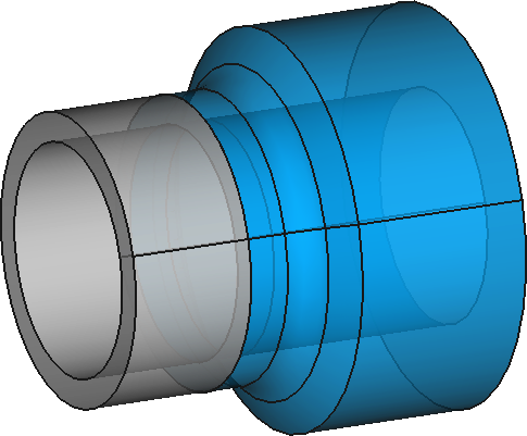{#fig:axi-inches-3d width=35%}

It consists of a typical vessel nozzle with attached piping as illustrated in\ [@fig:axi-inches-3d]. These components are subject to four transients\ $k=1,2,3,4$ that give rise to linearised stress histories (slightly modified according to NB-3216.2) which are given as individual stress values juxtaposed so as to span a time range of about 36,000 seconds ([@fig:nureg1]). As the time steps is not constant, each stress value has an integer index\ $i$ that uniquely identifies it:

$k$	Time range [s]	Index range	Cycles\ $n_k$
1	0--3210	1--523	20
2	3210--6450	524--959	50
3	6450--9970	960--1595	20
4	9970--35971	1596--2215	100

A design-basis earthquake was assumed to occur briefly during one second (sic) at around\ $t=3470$\ seconds, and it is assigned a number of cycles\ $n_e=5$. The detailed stress history for one of the SCLs including both the principal and lineariased stresses, which are already offset following NB-3216.2 so as to have a maximum stress equal to zero, can be found as an appendix in NRC’s NUREG/CR-6909 report, or in the repository with the scripts I prepared for you to play with this problem.

To compute the global usage factor, we first need to find all the combinations of local extrema pairs and then sort them in decreasing order of stress difference. For example, the largest stress amplitude is found between $i=447$ and $i=694$. The second one is 447--699. Then 699--1020, 699--899, etc. For each of these pairs, defined by the indexes\ $i{1,j}$ and $i{2,j}$, a partial usage factor\ $Uj$ should computed. The stress amplitude\ $S{\text{alt},j}$ which should be used to enter into the $S$-$N$ curve is

$$ S{\text{alt},j} = \frac{1}{2} \cdot k{e,j} \cdot \left| MB^\prime{i{1,j}} - MB^\prime{i{2,j}} \right| \cdot \frac{E\text{SN}}{E(T{\text{max}_j})} $$

\noindent where $ke$ is a plastic correction factor for large loads (NB-3228.5), $E\text{SN}$ is the Young’s Modulus used to create the $S$-$N$ curve (provided in the ASME fatigue curves) and\ $E(T_{\text{max}_j})$ is the material’s Young’s Modulus at the maximum temperature within the\ $j$-th interval.

We now need to comply with ASME’s obscure note about the number of cycles to assign a proper value of\ $n_j$. Back to the largest pair 447-694, we see that 447 belongs to transient\ #1 which has assigned 20 cycles and 694 belongs to the earthquake with 5 cycles. Therefore $n_1=5$, and the cycles associated to each index are decreased in five. So $i=694$ disappears and the number of cycles associated to $i=447$ are decreased from 20 to 15. The second largest pair is now 447-699, with 15 (because we just spent 5 in the first pair) and 50 cycles respectively. Now $n_2=15$, point 447 disappears and 699 remains with 35 cycles. The next pair is 699-1020, with number of cycles 35 and 20 so $n_3=20$, point 1020 disappears and 699 remains with 15 cycles. And so on, down to the last pair.

Why all these details? Not because I want to teach you how to perform fatigue evaluations just reading this section without resorting to ASME, fatigue books and even other colleagues. It is to show that even though these computation can be made “by hand” (i.e. using a calculator or, God forbids, a spreadsheet) when having to evaluate a few SCLs within several piping systems it is far (and I mean really far) better to automate all these steps by writing a set of scripts. Not only will the time needed to process the information be reduced, but also the introduction of human errors will be minimised and repeatability of results will be assured---especially if working under a distributed version control system such as Git. This is true in general, so here is another tip: learn to write scripts to post-process your FEM results (you will need to use a script-friendly FEM program) and you will gain considerable margins regarding time and quality.

::::: {#fig:nureg} {#fig:nureg1 width=70%}

{#fig:nureg2 width=70%}

{#fig:nureg3 width=70%}

:::::

:::::

:::::

:::::

:::::

:::::

:::::

:::::

:::::

:::::

:::::

:::::

:::::

:::::

:::::

:::::

:::::

:::::

:::::

:::::

:::::

:::::

:::::

:::::

:::::

:::::

:::::

:::::

::

::::: {#fig:cuf} 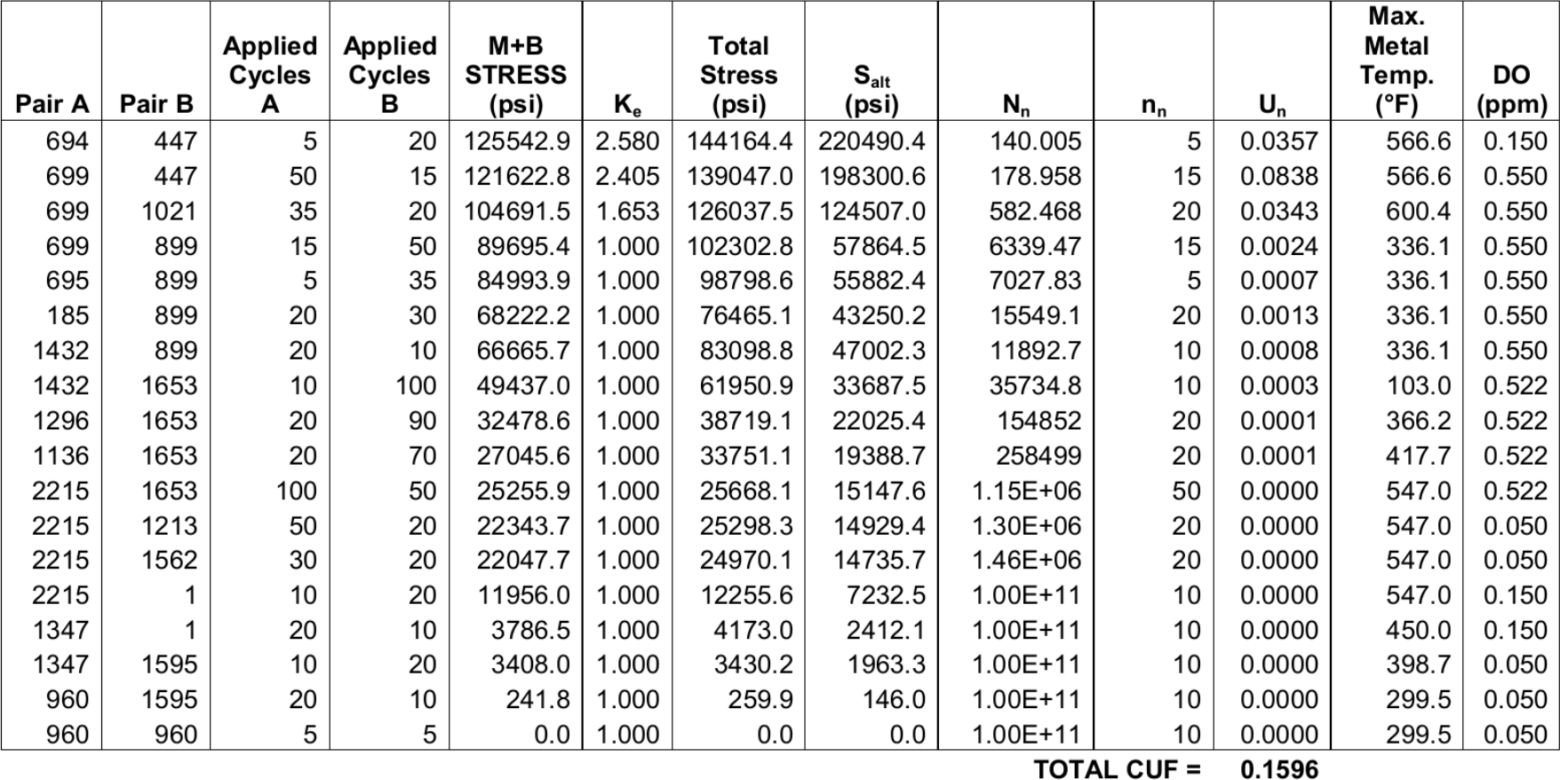{#fig:cuf-nrc width=100%}

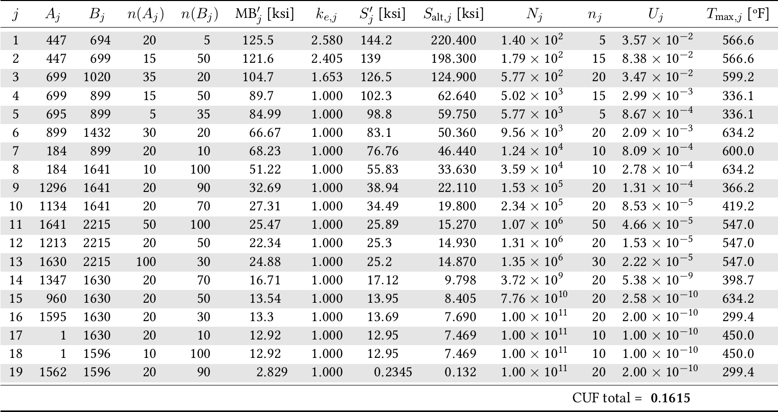{#fig:cuf-seamplex width=100%}

Tables of individual usage factors for the NRC/EPRI “EAF Sample Problem 2-Rev.\ 2 (10/21/2011).” One table is taken from a document issued by almost-a-billion-dollar-year-budget government agency from the most powerful country in the world and the other one is from a third-world engineering startup. Guess which is which. :::::

In water (NRC’s extension)

The fatigue curves and ASME’s (both\ III and\ VIII) methodology to analyse cyclic operations assume the parts under study are in contact with air, which is not the case of nuclear reactor pipes. Instead of building a brand new body of knowledge to replace ASME, the NRC decided to modify the former adding environmentally-assisted fatigue multipliers to the traditional usage factors, formally defined as

$$F\text{en} = \frac{N\text{air}}{N_\text{water}} \geq 1$$

This way, the environmentally-assisted usage factor for the $j$-th load pair is $\text{CUF}_\text{en,j} = Uj \cdot F{\text{en},j}$ and the global cumulative usage factor in water is the sum of these partial contributions

$$\text{CUF}_\text{en} = U1 \cdot F{\text{en},1} + U2 \cdot F{\text{en},2} + \dots + Uj \cdot F{\text{en},j} + \dots$${#eq:cufen}

In EPRI’s words, the general steps for performing an EAF analysis are as follows:

1. perform an ASME fatigue analysis using fatigue curves for an air environment
2. calculate $F_\text{en}$ factors for each transient pair in the fatigue analysis
3. apply the $F_\text{en}$ factors to the incremental usage calculated for each transient pair ($Uj$), to determine the $\text{CUF}\text{en}$, using\ [@eq:cufen]

Again, if $\text{CUF}\text{en} < 1$, then the system under study can withstand the assumed cyclic loads. Note that as\ $F{\text{en},j}$, we can have $\text{CUF} < 1$ and $\text{CUF}\text{en} > 1$ at the same time. The NRC has performed a comprehensive set of theoretical and experimental tests to study and analyse the nature and dependence of the non-dimensional correction factors\ $F\text{en}$. They found that, for a given material, they depend on:

a. the concentration\ $O(t)$ of dissolved oxygen in the water, b. the temperature\ $T(t)$ of the pipe, c. the strain rate\ $\dot{\epsilon}(t)$, and d. the content of sulphur\ $S(t)$ in the pipes (only for carbon or low-allow steels).

Apparently it makes no difference whether the environment is composed of either light or heavy water. There are somewhat different sets of non-dimensional analytical expressions that estimate the value of\ $F{\text{en}}(t)$ as a function of\ $O(t)$, $T(t)$, $\dot{\epsilon}(t)$ and $S(t)$, both in the few revisions of NUREG/CR-6909 and in EPRI’s report\ #1025823. Although they are not important now, the actual expressions should be defined and agreed with the plant owner and the regulator. The main result to take into account is that\ $F{\text{en}}(t)=1$ if\ $\dot{\epsilon}(t)\leq0$, i.e. there are no environmental effects during the time intervals where the material is being compressed.

Once we have the instantaneous factor\ $F{\text{en}}(t)$, we need to obtain an average value\ $F{\text{en},j}$ which should be applied to the\ $j$-th load pair. Again, there are a few different ways of lumping the time-dependent\ $F{\text{en}}(t)$ into a single $F{\text{en},j}$ for each interval. Both NRC and EPRI give simple equations that depend on a particular time discretisation of the stress histories that, in my view, are all ill-defined. My guess is that they underestimated their audience and feared readers would not understand the slightly-more complex mathematics needed to correctly define the problem. The result is that they introduced a lot of ambiguities (and even technical errors) just not to offend the maths illiterate. A decision I do not share, and a another reason to keep on learning and practising math.

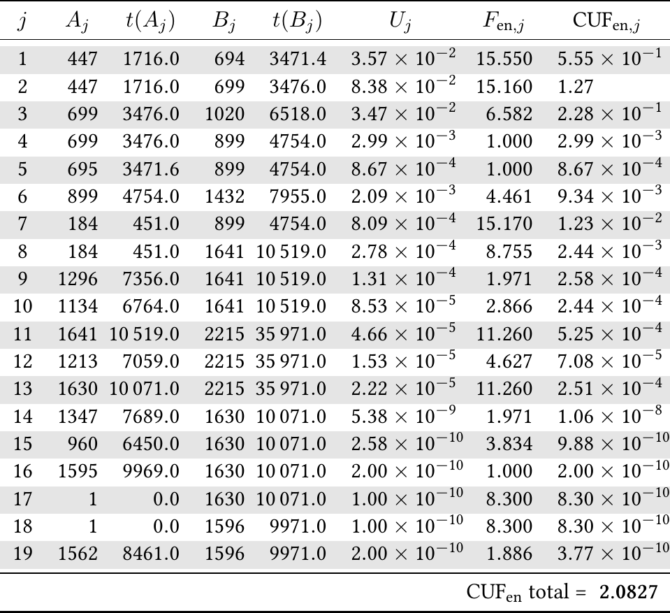
When faced for the first time with the case study, I have come up with a weighting method that I claim is less ill-defined (it still is for border-line cases) and which the plant owner accepted as valid. [@Fig:cufen] shows the reference results of the problem (based on computing two correction factors and then taking the maximum) and the ones obtained with the proposed method (by computing a weighted integral between the valley and the peak). Note how in\ [@fig:cufen-nrc], pairs 694-447 and 699-447 have the same\ $F_\text{en}$ even though they are (marginally) different. The results from\ [@fig:cufen-seamplex] give two (marginally) different correction factors.

::::: {#fig:cufen} 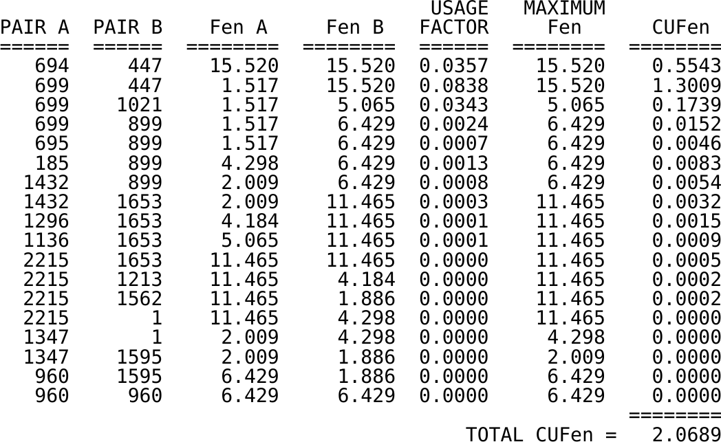{#fig:cufen-nrc width=75%}

{#fig:cufen-seamplex width=75%}

Tables of individual environmental correction and usage factors for the NRC/EPRI “EAF Sample Problem 2-Rev.\ 2 (10/21/2011).” The reference method assigns the same\ $F_\text{en}$ to the first two rows whilst the proposed lumping scheme does show a difference :::::