nafems4/nafems4.md

Background and introduction

First of all, please take this text as a written chat between you an me, i.e. an average engineer that has already taken the journey from college to performing actual engineering works using finite element analysis and has something to say about it. Picture yourself in a coffee bar, talking and discussing concepts and ideas with me. Maybe needing to go to a blackboard (or notepad?). Even using a tablet to illustrate some three-dimensional results. But always as a chat between colleagues.

Please also note that I am not a mechanical engineer, although I shared many undergraduate courses with some of them. I am a nuclear engineer with a strong background on mathematics and computer programming. I went to college between 2002 and 2008. Probably a lot of things have changed since then---at least that is what these “millennial” guys and girls seem to be boasting about---but chances are we all studied solid mechanics and heat transfer with a teacher using a piece of chalk on a blackboard while we as students wrote down notes with pencils on paper sheets. And there is really not much that one can do with pencil and paper regarding mechanical analysis. Any actual case worth the time of an engineer need to be more complex than an ideal canonical case with analytical solution.

Whether you are a student or a seasoned engineer with many years of experience, you might recall from first year physics courses the introduction of the simple pendulum as a case study\ ([@fig:simple]). You learned that the period does not depend on the hanging mass because the weight and the inertia exactly cancelled each other. Also, that Galileo said (and Newton proved) that for small oscillations the period does not even depend on the amplitude. Someone showed you why it worked this way: because if\ $\sin \theta \approx \theta$ then the motion equations converge to an harmonic oscillator. It might have been a difficult subject for you back in those days when you were learning physics and calculus at the same time. You might have later studied the Lagrangian and even the Hamiltonian formulations, added a parametric excitation and analysed the chaotic double pendulum. But it was probably after college, say when you took your first son to a swing on a windy day ([@fig:hamaca]), that you were faced with a real pendulum worth your full attention. Yes, this is my personal story but it could have easily been yours as well. My point is that the very same distance between what I imagined studying a pendulum was and what I saw that day at the swing (namely that the period does depend on the hanging mass) is the same distance between the mechanical problems studied in college and the actual cases encountered during a professional engineer’s lifetime ([@fig:pipes]). In this regard, I am referring only to technical issues. The part of dealing with clients, colleagues, bosses, etc. which is definitely not taught in engineering schools (you can get a heads up in business schools, but again it would be a theoretical pendulum) is way beyond the scope of both this article and my own capacities.

::::: {#fig:pendulum} {#fig:simple width=35%}\
{#fig:hamaca width=60%}

:::::

:::::

:::::

:::::

:::::

:::::

:::::

:::::

:::::

:::::

:::::

the swing’s period does depend on the hanging mass. See the actual video :::::

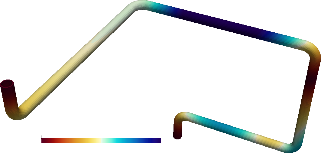
::::: {#fig:pipes} {#fig:infinite-pipe width=40%} {#fig:isometric width=58%}

An infinitely-long pressurised thick pipe as taught in college and an isometric drawing of a section of a real-life piping system :::::

Like the pendulums above, we will be swinging back and forth between a case study about fatigue assessment of piping systems in a nuclear power plant and more generic and even romantic topics related to finite elements and computational mechanics. These latter regressions will not remain just as abstract theoretical ideas. Not only will they be directly applicable to the development of the main case, but they will also apply to a great deal of other engineering problems tackled with the finite element method (and its cousins, [@sec:formulations]).

\medskip

Finite elements are like magic to me. I mean, I can follow the whole derivation of the equations, from the strong, weak and variational formulations of the equilibrium equations for the mechanical problem (or the energy conservation for heat transfer) down to the algebraic multigrid preconditioner for the inversion of the stiffness matrix passing through Sobolev spaces and the grid generation. Then I can sit down and program all these steps into a computer, including the shape functions and its derivatives, the assembly of the discretised stiffness matrix ([@sec:building]), the numerical solution of the system of equations ([@sec:solving]) and the computation of the gradient of the solution (@sec:stress-computation). Yet, the fact that all these a-priori unconnected steps give rise to pretty pictures that resemble reality is still astonishing to me.

Again, take all this information as coming from a fellow that has already taken such a journey from college’s pencil and paper to real engineering cases involving complex numerical calculations. And developing, in the meantime, both an actual working finite-element back-end and front-end from scratch.¹

Tips and tricks

There are some useful tricks that come handy when trying to solve a mechanical problem. Throughout this text, I will try to tell you some of them.

One of the most important ones to use your imagination. You will need a lot of imagination to “see” what it is actually going on when analysing an engineering problem. This skill comes from my background in nuclear engineering where I had no choice but to imagine a positron-electron annihilation or an spontaneous fission. But in mechanical engineering, it is likewise important to be able to imagine how the loads “press” one element with the other, how the material reacts depending on its properties, how the nodal displacements generate stresses (both normal and shear), how results converge, etc. And what these results actually mean besides the pretty-coloured figures.² This journey will definitely need your imagination. We will see equations, numbers, plots, schematics, CAD geometries, 3D\ views, etc. Still, when the theory says “thermal expansion produces normal stresses” you have to picture in your head three little arrows pulling away from the same point in three directions, or whatever mental picture you have about what you understand thermally-induced stresses are. What comes to your mind when someone says that out of the nine elements of the stress tensor ([@sec:tensor]) there are only six that are independent? Whatever it is, try to practice that kind of graphical thoughts with every new concept. Nevertheless, there will be particular locations of the text where imagination will be most useful. I will bring the subject up.

Another heads up is that we will be digging into some mathematics. Probably they would be be simple and you would deal with them very easily. But chances are you do not like equations. No problem! Just ignore them for now. Read the text skipping them, it should work as well. Łukasz Skotny says you do not need to know maths to perform finite-element analysis. And he is right, in the sense that you do not need to know thermodynamics to drive a car. It is fine to ignore maths for now. But, eventually, a time will come in which it cannot (or should not) be avoided. If you want to go to space, you will definitely have to learn thermodynamics.

So here comes another experience tip: do not fear equations. Even more, keep exercising. You have used differences of squares in high school, didn’t you?. You know (or at least knew) how to integrate by parts. Do you remember what Laplace transforms are used for? Once in a while, perform a division of polynomials using Ruffini’s rule. Or compute the second derivative of the quotient of two functions. Whatever. It should be like doing crosswords on the newspaper. Grab those old physics college books and read the exercises at the end of each chapter. It will pay off later on.

One final comment: throughout the text I will be referring to “your favourite FEM program.” I bet you do have one. Mine is CAEplex (it works on top of Fino). We will be using it to perform some tests and play a little bit. And we will also use it to think about what it means to use a FEM program to generate results that will eventually end up in a written project with your signature. Keep that in mind.

Case study: reactors, pipes and fatigue

Piping systems in sensitive industries like nuclear or oil & gas should be designed and analysed following the recommendations of an appropriate set of codes and norms, such as the ASME\ Boiler and Pressure Vessel Code. This code of practice was born during the late\ XIX century, before finite-element methods for solving partial differential equations were even developed. And much longer before they were available for the general engineering community. Therefore, much of the code assumes design and verification is not necessarily performed numerically but with paper and pencil (yes, like in college). However, it still provides genuine guidance in order to ensure pressurised systems behave safely and properly without needing to resort to computational tools. Combining finite-element analysis with the ASME code gives the cognisant engineer a unique combination of tools to tackle the problem of designing and/or verifying pressurised piping systems.

In the years following Enrico Fermi’s demonstration that a self-sustainable fission reaction chain was possible (actually, in fact, after WWII was over), people started to build plants in order to transform the energy stored within the atoms nuclei into usable electrical power. They quickly reached the conclusion that high-pressure heat exchangers and turbines were needed. So they started to follow codes of practise like the aforementioned ASME\ B&PVC. They also realised that some requirements did not fit the needs of the nuclear industry. But instead of writing a new code from scratch, they added a new chapter to the existing body of knowledge: the celebrated ASME Section\ III.

After further years passed by, engineers (probably the same people that forked section\ III) noticed that fatigue in nuclear power plants was not exactly the same as in other piping systems. There were some environmental factors directly associated to the power plant that were not taken into account by the regular ASME code. Again, instead of writing a new code from scratch, people decided to add correction factors to the previously-amended body of knowledge. This is how (sometimes) knowledge evolves, and it is this kind of complexities that engineers are faced with during their professional lives. We have to admit it, it would be a very difficult task to re-write everything from scratch every time something changes.

Actually, this article does not focus on a single case study but on some general ideas regarding analysis of fatigue in piping systems in nuclear power plants. There is no single case study but a compendium of ideas obtained by studying many different systems which are directly related to the safety of a real nuclear reactor.

{#fig:real-life}

Nuclear reactors

In each of the countries that have at least one nuclear power plant there exists a national regulatory body who is responsible for allowing the owner to operate the reactor. These operating licenses are time-limited, with a range that can vary from 25 to 60 years, depending on the design and technology of the reactor. Once expired, the owner might be entitled to an extension, which the regulatory authority can accept provided it can be shown that a certain (and very detailed) set of safety criteria are met. One particular example of requirements is that of fatigue in pipes, especially those that belong to systems that are directly related to the reactor safety.

Pressurised pipes

How come that pipes are subject to fatigue? Well, on the one hand and without getting into many technical details, the most common nuclear reactor design uses liquid water as coolant and moderator. On the other hand, nuclear power plants cannot by-pass the thermodynamics of the Carnot cycle, and in order to maximise the efficiency of the conversion of the energy stored in the uranium nuclei into electricity we need to reach temperatures as high as possible. So, if we want to have liquid water in the core as hot as possible, we need to increase the pressure. The limiting temperature and pressure are given by the critical point of water, which is around 374ºC and 22\ MPa. It is therefore expected to have temperatures and pressures near those values in many systems of the plant, especially in the primary circuit and those that directly interact with it, such as pressure and inventory control system, decay power removal system, feedwater supply system, emergency core-cooling system, etc.

Nuclear power plants are not always working at 100% of their maximum power capacity. They need to be maintained and refuelled, they may undergo operational (and some incidental) transients, they might operate at a lower power due to load following conditions, etc. These transient cases involve changes both in temperatures and in pressures that the pipes are subject to, which in turn give rise to changes in the stresses within the pipes. As the transients are postulated to occur cyclically during a number of times during the life-time of the plant (plus its extension period), mechanical fatigue in these piping systems may arise, especially at the interfaces between materials with different thermal expansion coefficients.

An important part of the analysis that almost always applies to nuclear power plants but usually also to other installations is the consideration of a possible seismic event. Given a postulated design earthquake, both the civil structures and the piping system itself need to be able to withstand such a load, even if it occurs at the moment of highest mechanical demand during one of the operational transients.

Fatigue

Mechanical systems can fail due to a wide variety of reasons. The effect known as fatigue can create, migrate and grow microscopic cracks at the atomic level, called dislocations. Once these cracks reach a critical size, then the material fails catastrophically even under stresses much lower than the tensile strength limits. There are not complete mechanistic models from first principles which can be used in general situations, and those that exist are very complex and hard to use. There are two main ways to approach practical fatigue assessment problems using experimental data very much like the Hooke’s Law experiment:

1. stress life, or
2. strain life

The first one is suitable for cases where the loads are nowhere near the yield stress of the material. When plastic deformation is expected to occur, strain-life methods ought to be employed.

For the case study, as the loads come principally from operational loads, the ASME\ stress-life approach should be used. The stress amplitude of a periodic cycle can be related to the number of cycles where failure by fatigue is expected to occur. For each material, this dependence can be computed using normalised tests and a family of “fatigue curves” like the one depicted in\ @fig:SN for different temperatures can be obtained.

{#fig:SN width=95%}

It should be noted that the fatigue curves are obtained in a particular load case, namely purely-periodic and one-dimensional, which cannot be directly generalised to other three-dimensional cases. Also, any real-life case will be subject to a mixture of complex cycles given by a stress time history and not to pure periodic conditions. The application of the curve data implies a set of simplifications and assumptions that are translated into different possible “rules” for composing real-life cycles. There also exist two safety factors which increase the stress amplitude and reduce the number of cycles respectively. All these intermediate steps render the analysis of fatigue into a conservative computation scheme ([@sec:kinds]). Therefore, when a fatigue assessment performed using the fatigue curve method arrives at the conclusion that “fatigue is expected to occur after ten thousand cycles” what it actually means is “we are sure fatigue will not occur before ten thousand cycles, yet it may not occur before one hundred thousand or even more.”

Solid mechanics, or what we are taught at college

So, let us start our journey. Our starting place: undergraduate solid mechanics courses. Our goal: to obtain the internal state of a solid subject to a set of movement restrictions and loads (i.e. to solve the solid mechanics problem). Our first step: Newton’s laws of motion. For our purposes, we can recall them here like this:

1. a solid is in equilibrium if it is not moving in at least one inertial coordinate system,
2. in order for a solid not to move, the sum of all the forces ought to be equal to zero, and
3. for every external load there exists an internal reaction with the same magnitude but opposite direction.

We have to accept that there is certain intellectual beauty when complex stuff can be expressed in such simple terms. Yet, from now on, everything can be complicated at will. We can take the mathematical path like D’Alembert and his virtual displacements ideas (in his mechanical treatise, he brags that he does not need to use a single figure throughout the book). Or we can go graphical following Culmann. Or whatever other logic reasoning to end up with a set of actual equations which we need to solve in order to obtain engineering results.

The stress tensor

In any case, what we should understand (and imagine) is that external forces lead to internal stresses. And in any three-dimensional body subject to such external loads, the best way to represent internal stresses is through a $3 \times 3$ stress tensor. This is the first point in which we should not fear mathematics. Trust me, it will pay back later on.

Does the term tensor scare you? It should not. A tensor is a general mathematical object and might get complex when dealing with many dimensions (as those encountered in weird stuff like string theory), but we will stick here to second-order tensors. They are slightly more complex than a vector, and I assume you are not afraid of vectors, are you? If you recall fresh-year algebra courses, a vector somehow generalises the idea of a scalar in the following sense: a given vector $\mathbf{v}$ can be projected into any direction $\mathbf{n}$ to obtain a scalar $p$. We call this scalar $p$ the “projection” of the vector $\mathbf{v}$ in the direction $\mathbf{n}$. Well, a tensor can be also projected into any direction $\mathbf{n}$. The difference is that instead of a scalar, a vector is now obtained.

Let me introduce then the three-dimensional stress tensor (a.k.a Cauchy tensor):

$$ \begin{bmatrix} \sigmax & \tau{xy} & \tau{xz} \ \tau{yx} & \sigma{y} & \tau{yz} \ \tau{zx} & \tau{zy} & \sigma_{z} \ \end{bmatrix} $$

It looks (and works) like a regular $3 \times 3$ matrix. Some brief comments about it:

• The $\sigma$s are normal stresses, i.e. they try to stretch or tighten the material.
• The $\tau$s are shear stresses, i.e. they try to twist the material.
• Due to rotational equilibrium requirements the conjugate shear stresses should be equal:
  • $\tau{xy} = \tau{yx}$,
  • $\tau{yz} = \tau{zy}$, and
  • $\tau{zx} = \tau{xz}$.

Therefore, the stress tensor is symmetric i.e. there are only six independent elements.

• The elements of the tensor depend on the orientation of the coordinate system.
• There exists a particular coordinate system in which the stress tensor is diagonal, i.e. all the shear stresses are zero. In this case, the three diagonal elements are called the principal stresses, which happen to be the three eigenvalues of the stress tensor. The basis of the coordinate system that renders the tensor diagonal are the eigenvectors.

What does this all have to do with mechanical engineering? Well, once we know what the stress tensor is for every point of a solid, in order to obtain the internal forces per unit area acting in a plane passing through that point and with a normal given by the direction $\mathbf{n}$, all we have to do is “project” the stress tensor through $\mathbf{n}$. In plain simple words:

If you can compute the stress tensor at each point of your geometry, then… Congratulations! You have solved the solid mechanics problem.

An infinitely-long pressurised pipe

Let us proceed to our second step, and consider the infinite pipe subject to uniform internal pressure already introduced in\ [@fig:infinite-pipe]. Actually, we are going to solve the mechanical problem on an infinite hollow cylinder, which looks like pipe. This case is usually tackled in college courses, and chances are you already solved it. In fact, the first (and simpler) problem is the “thin cylinder problem.” Then, the “thick cylinder problem” is introduced (the one we solve below), which is slightly more complex. Nevertheless, it has an analytical solution which is derived here. For the present case, let us consider an infinite pipe (i.e. a hollow cylinder) of internal radius $a$ and external radius $b$ with uniform mechanical properties---Young modulus $E$ and Poisson’s ratio $\nu$---subject to an internal uniform pressure $p$.

Displacements

Remember that when any solid body is subject to external forces, it has to react in such a way to satisfy the equilibrium conditions. The way solids do this is by deforming a little bit in such a way that the whole body acts as a compressed (or elongated) spring balancing the load. So it is worth to ask how a pressurised pipe deforms to counteract the internal pressure\ $p$.

• There are no longitudinal displacements\ $u_l$ because the pipe is infinite in the axial direction.
• There are no azimuthal displacements\ $u_\theta$ because the pipe is fully symmetric around the axis.
• There are only radial displacements\ $u_r$ and they depend only on the radial coordinate\ $r$ and not on the axial position\ $z$ or on the azimuthal angle\ $\theta$. These displacements are

$$ u_r® = p \cdot \frac{1+\nu}{E} \cdot \frac{a^2}{b^2-a^2} \cdot \left[ 1-2\nu + \frac{b^2}{r^2} \right]\cdot r $$

What does this mean? Well, that overall the whole pipe expands a little bit radially with the inner face being displaced more than the external surface (use your imagination!). How much?

1. linearly with the pressure, i.e. twice the pressure means twice the displacement, and
2. inversely proportional to the Young Modulus\ $E$ divided by $1+\nu$, i.e. the more resistant the material, the less radial displacements.

That is how an infinite pipe withstands internal pressure.

Stresses

As the solid is deformed, that is to say that different parts are relatively displaced one from another, strains and stresses appear. When seen from a cylindrical coordinate system, the stress tensor (recall [@sec:tensor]) has these features.

• There are no shear stresses as there is no bending due to the fact that the pipe is infinite (so it cannot bend in the axial direction) and azimuthally symmetric (there is no particular direction so circles must remain circles).

• The normal stresses depend only on the radial coordinate\ $r$ and are

  • the radial stress\ $\sigma_r$,

  $$ \sigma_r® = \frac{p \cdot a^2}{b^2-a^2} \cdot \left( 1 - \frac{b^2}{r^2}\right) $$ {#eq:sigmar}

  • the azimuthal (or hoop) stress\ $\sigma_\theta$, and

  $$ \sigma_\theta® =\frac{p \cdot a^2}{b^2-a^2} \cdot \left( 1 + \frac{b^2}{r^2}\right) $$ {#eq:sigmatheta}

  • the longitudinal (or axial) stress\ $\sigma_l$.

  $$ \sigma_l® = 2\nu \cdot \frac{p \cdot a^2}{b^2-a^2} $${#eq:sigmal}

We can note that

1. The stresses do not depend on the mechanical properties\ $E$ and\ $\nu$ of the material (the displacements do).
2. All the stresses are linear with the pressure\ $p$, i.e. twice the pressure means twice the stress.
3. The axial stress is uniform and does not depend on the radial coordinate\ $r$.
4. As the stress tensor is diagonal, these three stresses happen to also be the principal stresses.

That is all what we can say about an infinite pipe with uniform material properties subject to an uniform internal pressure\ $p$. If

• the pipe was not infinite (say any real pipe that has to start and end somewhere), or
• the cross-section of the pipe is not constant along the axis (say there is an elbow or even a reduction), or
• there was more than one pipe (say there is a tee), or
• the material properties are not uniform (say the pipe does not have an uniform temperature but a distribution), or
• the pressure was not uniform (say because there is liquid inside and its weight cannot be neglected),

\noindent then we would no longer be able to fully solve the problem with paper and pencil and draw all the conclusions above. However, at least we have a start because we know that if the pipe is finite but long enough or the temperature is not uniform but almost, we still can use the analytical equations as approximations. After all, Enrico Fermi managed to reach criticality in the Chicago Pile-1 with paper and pencil. But what happens if the pipe is short, there are branches and temperature changes like during a transient in a nuclear reactor? Well, that is why we have finite elements. And this is where what we learned at college pretty much ends.

Finite elements, or solving actual problems

Besides infinite pipes (both thin and thick), spheres and a couple of other geometries, there are no other cases for which we can obtain analytical expressions for the elements of the stress tensor. To get results for a solid with real engineering interest, we need to use numerical methods to solve the equilibrium equations. It is not that the equations are hard per se. It is that the mechanical parts we engineers like to design (which are of course more complex than cylinders and spheres) are so intricate that render simple equations into monsters which are unsolvable with pencil and paper. Hence, finite elements enter into the scene.

The name of the game

But before turning our attention directly into finite elements (and leaving college, at least undergraduate) it is worth some time to think about other alternatives. Are we sure we are tackling your problems in the best possible way? I mean, not just engineering problems. Do we take a break, step back for a while and see the whole picture looking at all the alternatives so we can choose the best cost-effective one?

There are literally dozens of ways to numerically solve the equilibrium equations, but for the sake of brevity let us take a look at the three most famous ones. Coincidentally, they all contain the word “finite” in their names. We will not dig into them, but it is nice to know they exist. We might use

1. Finite differences
2. Finite volumes
3. Finite elements

Each of these methods (also called schemes) have of course their own features, pros and cons. They all exploit the fact that the equations are easy to solve in simple geometries (say a cube). Then the actual geometry is divided into a juxtaposition of these cubes, the equations are solved in each one and then a global solution is obtained by sewing the little simple solutions one to another. The process of dividing the original domain into simple geometries is called discretisation, and the resulting collection of these simple geometries is called a mesh or grid. They are composed of volumes, called cells (or elements) and vertices called nodes. Now, grids can be either

a. structured, or b. unstructured

Figure [-@fig:grids] illustrates how the same domain can be discretised using these two kind of grids. In the first case, we could identify any single cell by using just two indexes. We could even tell which nodes define each cell just from these indexes. In the second case, we need an explicit list just to know how many cells there are. Even more, there is no way to link the nodes with the cells (back and forth) other than having an explicit list of nodes and cells. Again, there are pros and cons for each of the grid types such as simplicity, flexibility, etc. In general, unstructured grids can better represent a certain geometry with the same number of cells. Structured grids suffer the so-called “staircase effect” that makes the unusable for discretising mechanical parts.

::::: {#fig:grids} {#fig:continuous width=30%}\
{#fig:structured width=30%}\
{#fig:unstructured width=30%}

Discretisation of a spatial domain, For the same number of cells, unstructured grids can better represent arbitrary shapes. :::::

Back to the three numerical methods, we must say that finite differences is based on approximating derivatives (i.e. differentials) by incremental quotients (i.e. differences). The second one heavily relies on geometrical ideas rather than on pure mathematical grounds. Finally, our beloved finite elements are more strict in the mathematical sense. Actually, a complete derivation of the finite element method can be written in a textbook without requiring a single figure, just like D’Alembert did more than two centuries ago. In any case, it is important to note that finite differences and elements compute results at the nodes of a mesh, whilst finite volumes compute results at the cells of a mesh. Finally, any method may be used in structured grids but only finite elements and volumes are especially suited for working with unstructured grids.

There are technical reasons that justify why the finite element method is the king of mechanical analysis. But that does not mean that other methods may be employed. For instance, fluid mechanics are generally better solved using finite volumes. And further other combinations may be found in the literature.

Before proceeding, I would like to make two comments about common nomenclature. The first one is that if we exchanged the words “volumes” and “elements” in all the written books and articles, nobody would notice the difference. There is nothing particular in both theories that can justify why FVM use “volumes” and FEM use “elements”. Actually volumes and elements are the same geometric constructions. As far as I know, the names were randomly assigned.

The second one is more philosophical and refers to the word “simulation” which is often used to refer to solving a problem using a numerical scheme such as the finite element method. I am against at using this word for this endeavour. The term simulation has a connotation of both “pretending” and “faking” something, that is definitely not what we are doing when we solve an engineering problem with finite elements. Sure, there are some cases in which we simulate, such as using the Monte Carlo method (originally used by Fermi as an attempt to understand how neutrons behave in the core of nuclear reactors). But when solving deterministic mechanical engineering problems I would rather say “modelling” than “simulation.”

Kinds of finite elements

This section is not (just) about different kinds of elements like tetrahedra, hexahedra, pyramids and so on. It is about the different kinds of analysis there are. Indeed, there is a whole plethora of particular types of calculations we can perform, all of which can be called “finite element analysis.” For instance, for the mechanical problem, we can have different kinds of

• temporal dependence
  • steady-state
  • quasi-static
  • transient
• main elements
  • 1D beam elements
  • 2D shell elements
  • 3D bulk elements
• mathematical models
  
  • pure linear
  • material non-linear
  • geometrical non-linear
• particular studies
  • buckling
  • modal
• element features
  • isoparametric elements
  • serendipity elements
  • sub-integrated elements
  • incomplete elements

And then there exist different pre-processors, meshers, solvers, pre-conditioners, post-processing steps, etc. A similar list can be made for the heat conduction problem, electromagnetism, the Schröedinger equation, neutron transport, etc. But there is also another level of “kind of problem,” which is related to how much accuracy and precision we are to willing sacrifice in order to have a (probably very much) simpler problem to solve. Again, there are different combinations here but a certain problem can be solved using any of the following three approaches, listed in increasing amount of difficulty and complexity:

i. conservative ii. best-estimate iii. probabilistic

The first one is the easiest because we are allowed to choose parameters and to make engineering decisions that may simplify the computation as long as they give results towards the worst-case scenario. More often than not, a conservative estimation is enough in order to consider a problem as solved. Note that this is actually how fatigue results are obtained using fatigue curves, as discussed in\ [@sec:fatigue]. A word of care should be taken when considering what the “worst-case scenario” is. For instance, if we are analysing the temperature distribution in a mechanical part subject to convection boundary conditions, we might take either a very large or a very low convection coefficient as the conservative case. If we needed to design fins to dissipate heat then a low coefficient would be the conservative choice. But if the mechanical properties deteriorated with high temperatures then the conservative way to go would be to set a high convection coefficient. A common practice is to have a fictitious set of parameters, each of them being conservative leading individually to the worst case even if the overall combination is not physically feasible.

As neat and tempting as conservative computations may be, sometimes the assumptions may be too biased toward the bad direction and there might be no way of justifying certain designs with conservative computations. It is then time to sharpen our pencils and perform a best-estimate computation. This time, we should stick to the most-probable values of the parameters and even use more complex models that can better represent the physical phenomena that are going on in our problem. Sometimes best-estimate computations are just slightly more complex than conservative models. But more often than not, best-estimates get far more complicated. And these complications come not just in the finite-element model of the elastic problem but in the dependence of properties with space, time and/or temperature, in non-trivial relationships between macro and microscopic parameters, in more complicated algorithms for post-processing data, etc.

Finally, when then uncertainties associated to the parameters, methods and models used in a best-estimate calculation render the results too inaccurate, it might be needed to do a full set of parametric runs taking into account the probabilistic distribution of each of the input parameters. It involves

1. a thorough analysis of the probability densities of the parameters (and even the methods) of a problem,
2. performing a large number of runs for different combination of parameters, and
3. combining all the results into to obtain a best-estimate value plus uncertainty.

This kind of computation is usually required by the nuclear regulatory authorities when power plant designers need to address the safety of the reactors. What is the heat capacity of uranium above 1000ºC? What is the heat transfer coefficient when approaching the critical heat flux before the Leidenfrost effect occurs? A certain statistical analysis has to be done prior to actually parametrically sweeping (see\ [@sec:parametric]) the input parameters so as to obtain a distribution of possible outcomes.

Five whys

So we know we need a numerical scheme to solve our mechanical problem because anything slightly more complex than an infinite pipe does not have analytical solution. We need an unstructured grid because we would not use Legos to discretise cylindrical pipes. We selected the finite elements method over the finite volumes method, because FEM is the king. Can we pause again and ask ourselves why is it that we want to do finite-element analysis?

\medskip

There exists a very useful problem-solving technique conceived by Taiichi Ohno, the father of the Toyota production system, known as the Five-whys rule. It is based on the fact people make decisions following a certain reasoning logic that most of the time is subjective and biased, and not purely rational and neutral. By recursively asking (at least five times) the cause of a certain issue, it might possible to understand what the real nature of the problem (or issue being investigated) is. And it might even be possible to to take counter-measures in order to fix what seems wrong.

Here is the original example:

1. Why did the robot stop?
   The circuit has overloaded, causing a fuse to blow.

2. Why is the circuit overloaded?
   There was insufficient lubrication on the bearings, so they locked up.

3. Why was there insufficient lubrication on the bearings?
   The oil pump on the robot is not circulating sufficient oil.

4. Why is the pump not circulating sufficient oil?
   The pump intake is clogged with metal shavings.

5. Why is the intake clogged with metal shavings?
   Because there is no filter on the pump.

You get the point, even though we know thanks to Richard Feynmann that to answer a “why” question at some point we need to rely on the questioner’s previous experience. We usually assume we have to do what we usually do (i.e. perform finite element analysis). But do we? Do we add a filter or do we just replace the fuse?

\medskip

Getting back to the case study: do we need to do FEM analysis? Well, it does not look like we can obtain the stresses of the transient cycles with just pencil and paper. But how much complexity should we add? We might do as little as axisymmetric linear steady-state conservative studies or as much as full three-dimensional non-linear transient best-estimate plus uncertainties computations. And here is where good engineers stand out: in putting their engineering judgment (call it experience or hunches) into defining what to solve. And it is not (just) because the first option is faster to solve than the latter. Involving many complex methods need more engineering time

1. to prepare the input data and set up the algorithms,
2. to cope with the many more mistakes that will inevitable appear during the computation, and
3. to analyse the output data and write engineering reports.

In the first years of the history of computers, when programs were written in decks and output results were printed in continuous paper sheets, it made sense for computer programs to calculate and write as much data as possible even if it was not needed. One would never know if it would not be needed in the future, and CPU time was so expensive that re-running engineering computations because a particular result was not included in the output was forbidden. But that is not remotely true in the XXI century anymore. Computing time is far cheaper than engineering time (result known as the UNIX Rule of Economy) that it should be neglected with respect to the time spent by a cognisant engineer searching and sorting thousands of hard-to-read floating-point numbers.

divert(-1)

---

Computers, those little magic boxes

When we think about finite elements, we automatically think about computers. Of

https://www.springfieldspringfield.co.uk/view_episode_scripts.php?tv-show=the-simpsons&episode=s05e03

ENIAC

A brief review of history

FEM, Computers

graphics cards

Hardware

Software

FOSS

Avoid black boxes

Reflections on trusting trust

UNIX, scriptability, make programs to make programs (here a program is a calculation)

front and back

avoid monolithic

---

divert(0)

Piping in nuclear rectors

So we need to address the issue of fatigue in nuclear reactor pipes that

1. are not infinite and have cross-section changes, branches, valves, etc.
2. are made of different materials,
3. are fixed at different locations through piping supports,
4. are subject to a. pressure transients, b. heat transients, and c. seismic loads.

As I wanted to illustrate in [@sec:five], it is very important to decide what kind of problem (actually problems) we should be dealing with. As a nuclear engineer, I learned (theoretically in college but practically after college) that there are some models that let you see some effects and some that let you see other effects (please say “modelling” not “simulation.”). And even if, in principle, it is true that more complex models should let you see more stuff, they definitely might show you nothing at all if the model is so big and complex that it does not fit into a computer (say because it needs hundreds of gigabytes of RAM to run) or because it takes more time to compute than you may have before the final report is expected.

First of all, we should note that we need to solve

i. the heat transfer equation to get the temperature distribution within the pipes, ii. the natural frequencies and oscillation modes of the piping system to obtain the pseudo-accelerations generated by the design earthquake, and finally iii. the elastic problem to obtain the stress tensor needed to compute the alternating stress to enter into the fatigue curve.

So for each time\ $t$ of the operational transient, the pipes are subject to

a. an uniform internal pressure\ $p_i(t)$ that depends on time, b. a non-uniform internal temperature $T_i(t)$ that gives rise to a non-trivial time-dependent temperature distribution\ $T(\mathbf{x},t)$ in the bulk of the pipes, and c. internal distributed forces\ $\mathbf{f}=\rho \cdot \mathbf{a}$ at those times where the design earthquake is assumed to occur.

Thermal transient

Let us invoke our imagination once again. Assume in one part of the transients the temperature of the water inside the pipes falls from say 300ºC down to 100ºC in a couple of minutes, stays at 100ºC for another couple of minutes and then gets back to 300ºC. The temperature within the bulk of the pipes changes as times evolves. The internal wall of the pipes follow the transient temperature (it might be exactly equal or close to it through the Newton’s law of cooling). If the pipe was in a state of uniform temperature, the ramp in the internal wall will start cooling the bulk of the pipe creating a transient thermal gradient. Due to thermal inertia effects, the temperature can have a non-trivial dependence when the ramps start or end (think about it!). So we need to compute a real transient heat transfer problem with convective boundary conditions because any other usual tricks like computing a sequence of steady-state computations for different times would not be able to recover these non-trivial distributions.

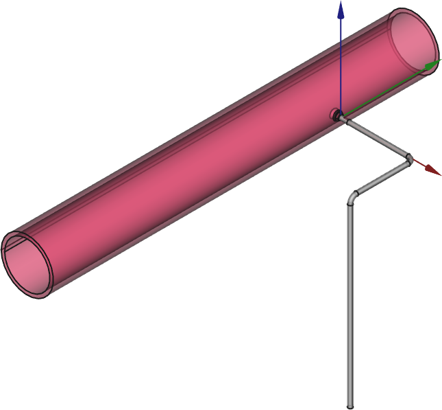
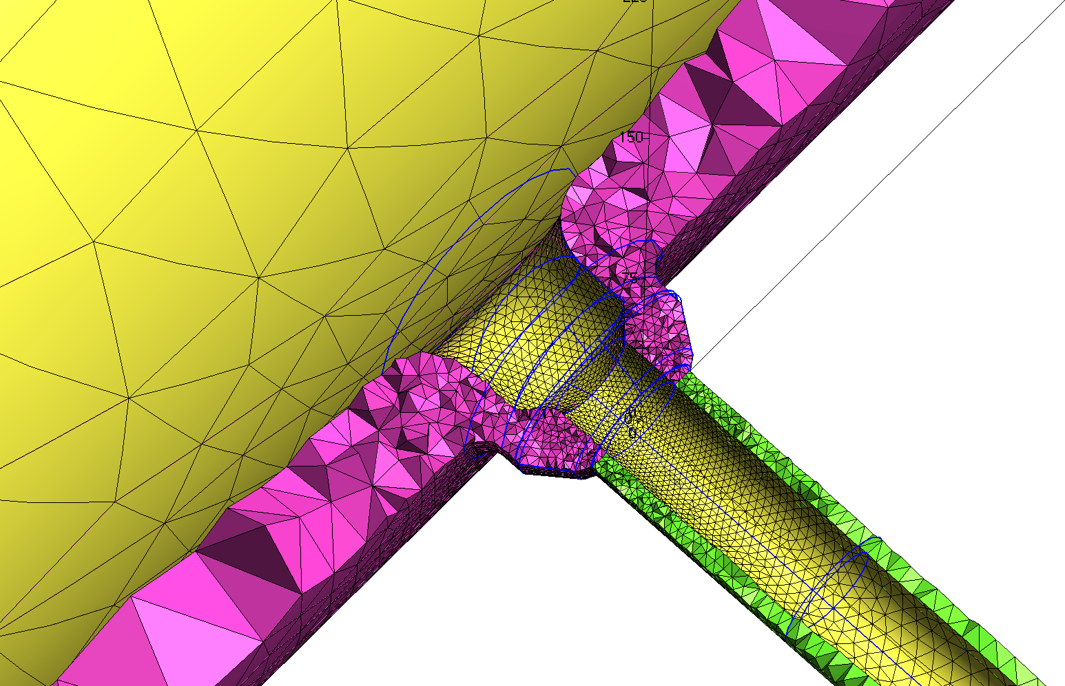
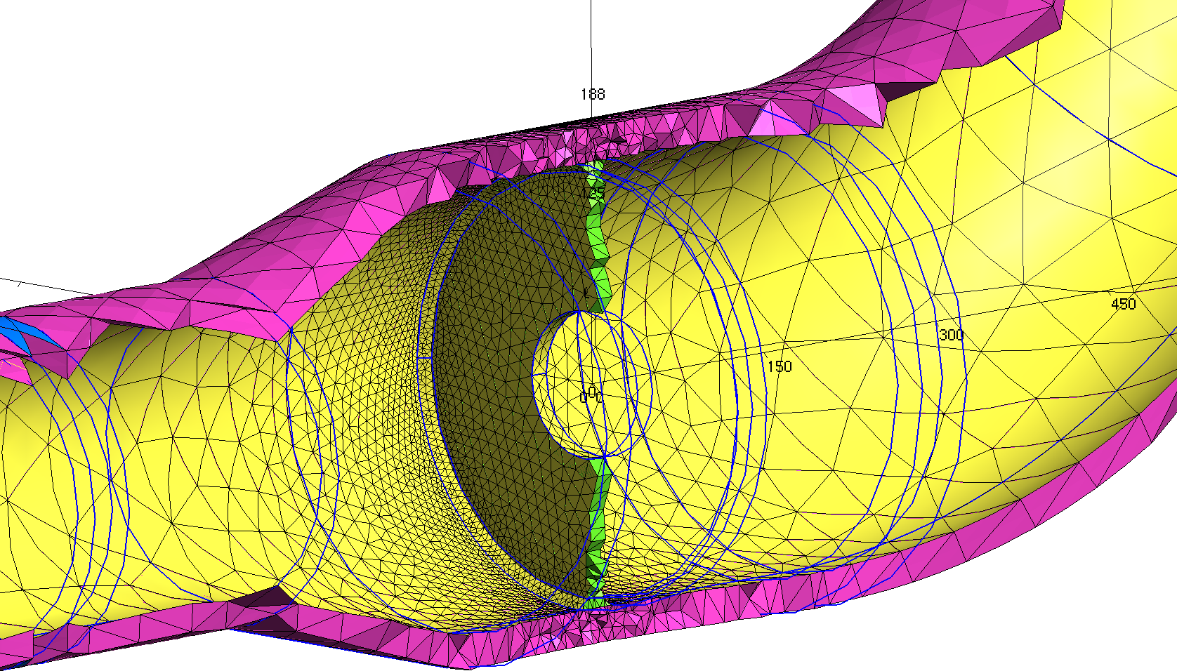
Remember the main issue of the fatigue analysis in these systems is to analyse what happens around the location of changes of piping classes where different materials (i.e. different expansion coefficients) are present, potentially causing high stresses due to differential thermal expansion (or contraction) under transient conditions. Therefore, even though we are dealing with pipes we cannot use beam or circular shell elements, because we need to take into account the three-dimensional effects of the temperature distribution along the pipe thickness. And even if we could, there are some tees that connect pipes with different nominal diameters that have a non-trivial geometry, such as the weldolet-type junction shown in\ [@fig:weldolet-cad;@fig:weldolet-mesh]. In this case, there are a number of SCLs (Stress Classification Lines) that go through the pipe’s thickness at both sides of the material interface as illustrated in\ [@fig:weldolet-scls]. It is in these locations that fatigue is to be evaluated.

dnl 33410 07-3-4D-29

::::: {#fig:weldolet-cad} {#fig:weldolet-cad1 width=80%}

{#fig:weldolet-cad2}

CAD model of a piping system with a ¾-inch weldolet-type fork (stainless steel) from a main 12-inch pipe (carbon steel) :::::

::::: {#fig:weldolet-mesh} {#fig:weldolet-mesh1 width=55%}

{#fig:weldolet-mesh2}

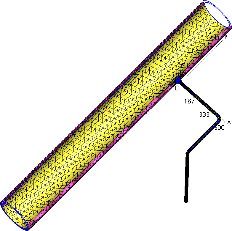
Three-dimensional unstructured tetrahedra-based grid for the system shown in\ [@fig:weldolet-cad] :::::

{#fig:weldolet-scls width=75%}

On the one hand, a reasonable number of nodes (it is the number of nodes that defines the problem size, not the number of elements as discussed in [@sec:elements-nodes]) in order to get a decent grid is around 200k for each system. On the other hand, solving a couple of dozens of transient heat transfer problems (which we cannot avoid due to the large thermal inertia of the pipes) during a few thousands of seconds over a couple hundred of thousands of nodes might take more time and storage space to hold the results than we might expect.

There is a wonderful essay by Isaac Asimov called “The Relativity of Wrong” where he introduces the idea that even if something cannot be computed exactly, there are different levels of error. For instance, believing that the Earth is a sphere is less wrong than believing that the Earth is flat, but wrong nonetheless, since it really deviates from a perfect sphere and resembles more an oblate spheroid.

We can then merge this idea by Asimov with an adapted version of the Saint-Venant’s principle and note that the detailed transient temperature distribution is important only around the location of the SCLs. We can then make an engineering approximation and

1. compute the transient thermal problem using a reduced mesh around the SCLs, and
2. assume the part of the full system which is not contained in the reduced mesh is at an uniform (though not constant) temperature equal to the average of the inner and outer temperatures at each side of the reduced mesh.

dnl 33300 02-D-3-4

::::: {#fig:valve} {#fig:valve-cad1 width=75%}

{#fig:valve-mesh1 width=75%}

{#fig:valve-scls1 width=60%}

An example case where the SCLs are located around the junction between stainless-steel valves and carbon steel pipes at both sides of the material interface in the vertical plane both at the top and at the bottom of the pipe :::::

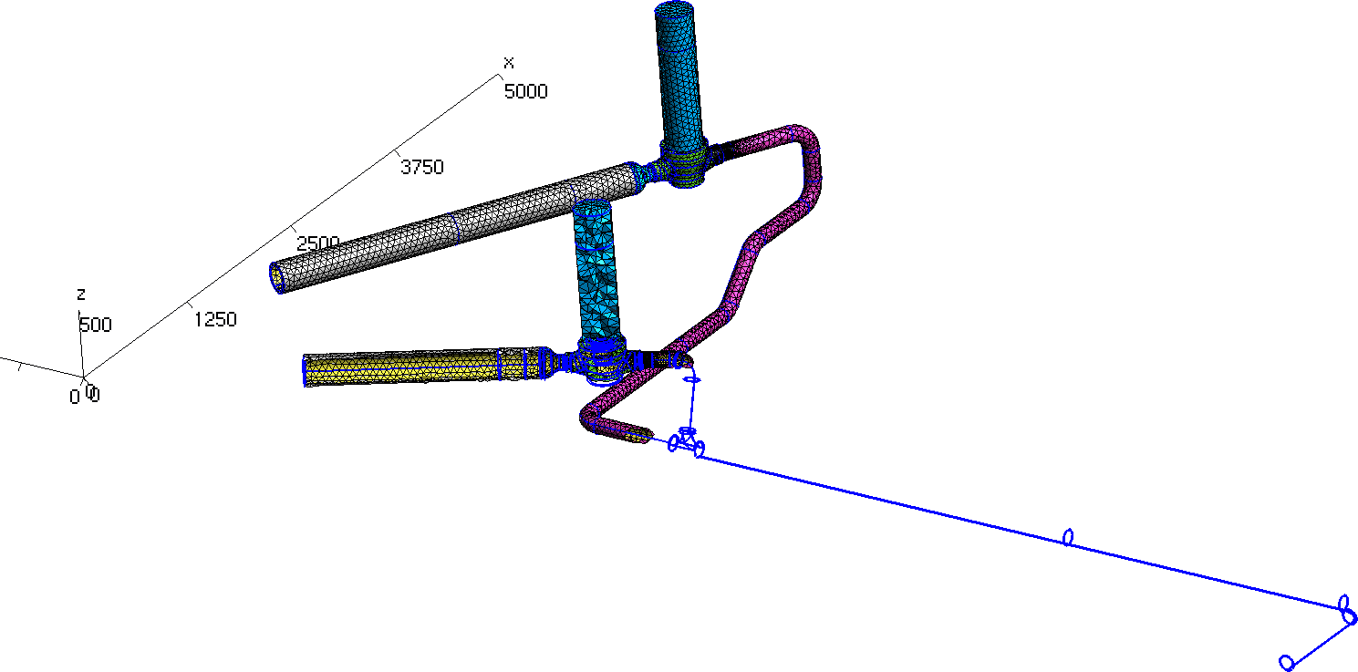
As an example, let us consider the system depicted in\ [@fig:valve] where there is a stainless-carbon steel interface at the discharge of the valves. Instead of solving the transient heat-conduction problem with the internal temperature of the pipes equal to the temperature of the water in the reference transient condition of the power plant and an external condition of natural convection to the ambient temperature in the whole mesh of\ [@fig:valve-mesh1], a reduced model consisting of half of one of the two valves and a small length of the pipes at both the valve inlet and outlet is used. Once the temperature distribution\ $\hat{T}(\mathbf{x},t)$ for each time is obtained in the reduced mesh ([@fig:valve-temp], which has the origin at the centre of the valve), the actual temperature distribution\ $T(\mathbf{x},t)$ is computed by an algebraic generalisation of $\hat{T}(\mathbf{x},t)$ in the full coordinate system (where the origin is shown in\ [@fig:valve-cad1]). As stated above, those locations which are not covered by the reduced model are generalised with a time-dependent uniform temperature which is the average of the inner and outer temperatures at the inlet and outlet of the reduced mesh. The result is illustrated in figure\ [@fig:valve-gen].

::::: {#fig:valve-temp-gen} 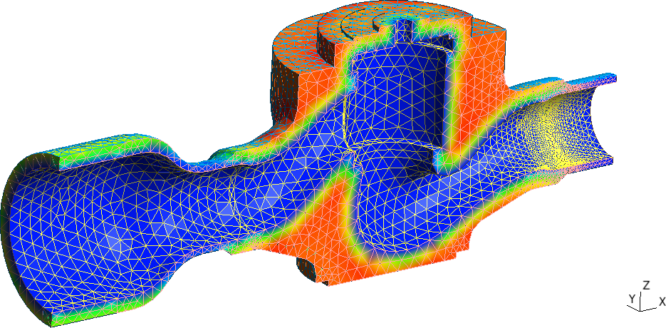{#fig:valve-temp width=80%}

{#fig:valve-gen width=95%}

Computation of the thermal problem in a reduced mesh and generalisation of the result to the full original 3D mesh of figure\ [@fig:valve-mesh1] :::::

Note that there is no need to have a one-to-one correspondence between the elements from the reduced mesh with the elements from the original one. Actually, the reduced mesh contains first-order elements whilst the former has second-order elements. Also the grid density is different. Nevertheless, the finite-element solver Fino used to solve both the heat and the mechanical problems, allows to read functions of space and time defined over one mesh and continuously evaluate and use them into another one even if the two grids have different elements, orders or even dimensions. In effect, in the system from\ [@fig:real-life] the material interface is between a orifice plate made in stainless steel that is welded to a carbon-steel pipe ([@fig:real-mesh2]). The thermal problem can be modelled using a two-dimensional axi-symmetric grid [@fig:real-temp] and then generalised to the full three-dimensional mesh using the algebraic manipulation capabilities provided by Fino (actually by wasora) as shown in\ [@fig:real-gen].

dnl 33410 10-12D-24

::::: {#fig:real} {#fig:real-mesh2 width=70%}

{#fig:real-temp width=100%}

{#fig:real-gen width=75%}

The material interface in the system from [@fig:real-life] is configured by an orifice plate made of stainless steel welded to a carbon-steel pipe :::::

Seismic loads

Before considering the actual mechanical problem that will give us the stress tensor at the SCLs, and besides needing to solve the transient thermal problem to get the temperature distributions, we need to address the loads that arise due to a postulated earthquake during a certain part of the operational transients. The full computation of a mechanical transient problem using the earthquake time-dependent displacements is off the table for two reasons. First, because again the computation would take more time than we might have to deliver the report. And secondly and more importantly, because civil engineers do not compute earthquakes in the time domain but in the frequency domain using the response spectrum method. Time to revisit our Fourier transform exercises from undergraduate maths courses.

Earthquake spectra

Every nuclear power plant is designed to withstand earthquakes. Of course, not all plants need the same level of reinforcements. Those built in large quiet plains will be, seismically speaking, cheaper than those located in geologically active zones. Keep in mind that all the 54 Japanese nuclear power plants did structurally resist the 2011 earthquake, and all of the reactors were safely shut down. What actually happened in Fukushima is that one hour after the main shake, a 14-metre tsunami splashed on the coast, jumping over the 9-metre defences and flooding the emergency Diesel generators that provided power to the pumps in charge of removing the remaining decay power from the already-stopped reactor core.

Back to our case study, the point is that each site where nuclear power plants are built must have a geological study where a postulated design-basis earthquake is to be defined. In other words, a theoretical earthquake which the plant ought to withstand needs to be specified. How? By giving a set of three spectra (one for each coordinate direction) giving acceleration as a function of the frequency for each level of the building. That is to say, once the earthquake hits the power plant, depending on soil-structure interactions the energy will shake the building foundations in a way that depends on the characteristics of the earthquake, the soil and the concrete structure. Afterwards, the way the oscillations travel upward and shake each of the mechanical components erected in each floor level depends on the design of the civil structure in a way which is fully determined by the floor response spectra like the ones depicted in\ [@fig:spectrum].

{#fig:spectrum width=90%}

Natural frequencies

As the earthquake excites some frequencies more than others, it is mandatory to know which are the natural frequencies and modes of oscillations of our piping system. Mathematically, this requires the computation of an eigenvalue problem. Simply stated, we need to find all the non-trivial solutions of the equation

$$ K \phi_i = \lambda_i \cdot M \phi_i $$ where $K$ is the usual finite-element stiffness matrix, $M$ is the mass matrix, $\lambda_i$ is the $i$-th natural frequency of the structure and $\phi_i$ is a vector containing the nodal displacement corresponding to the $i$-th mode of oscillation.

Practically, these problems are solved using the same mechanical finite-element program one would use to solve a standard elastic problem, provided such program supports these kind of problems (Fino does). There are only two caveats we need to take into account:

1. The computation of the natural frequencies is “load free”, i.e. there can be no surface nor volumetric loads, and
2. The displacement boundary conditions ought to be homogeneous, i.e. only displacements equal to zero can be given. We may fix only one of the three degrees of freedom in certain surfaces and leave the others free, as long as all the rigid body motions are removed as usual.

A real continuous solid has infinite modes of oscillation. A discretised one (using the most common and efficient FEM formulation, the displacement-based formulation) has three times the number of nodes modes. In any case, one is usually interested only in a few of them, namely those with the lower frequencies because they take away most of the energy with them. Each mode has two associated parameters called modal mass and excitation that reflect how “important” the mode is regarding the absorption of energy from an external oscillatory source. Usually a couple of dozens of modes are enough to take up more than 90% of the earthquake energy. Figure\ [-@fig:modes] shows the first six natural modes of a sample piping section.

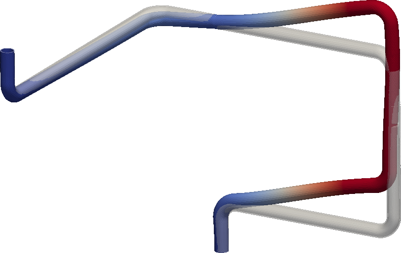
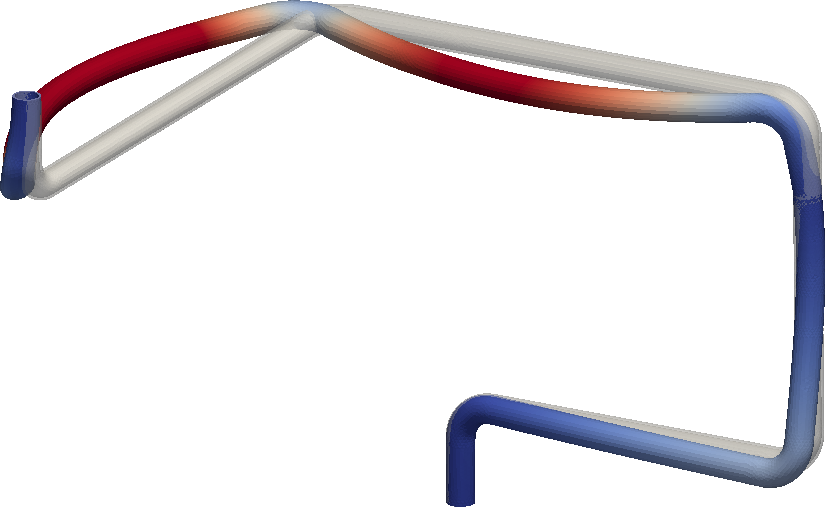
::::: {#fig:modes} {width=48%}\
{width=48%}

{width=48%}\
{width=48%}

{width=48%}\
{width=48%}

First six natural oscillation modes for a piping section :::::

These first modes that take up most of the energy are then used to take into account the earthquake load. There are several ways of performing this computation, but the ASME\ III code states that the method known as SRSS (for Square Root of Sum of Squares) can be safely used. This method mixes the eigenvectors with the floor response spectra through the eigenvalues and gives a spatial (actually nodal) distribution of three accelerations (one for each direction) that, when multiplied by the density of the material, give a vector of a distributed force (in units of Newton per cubic millimetre for example) which is statically equivalent to the load coming from the postulated earthquake.

::::: {#fig:acceleration} {width=80%}

{width=80%}

{width=80%}

The equivalent accelerations for the piping section of [@fig:modes] for the spectra of\ [@fig:spectrum] :::::

The ASME code says that these accelerations (depicted in [@fig:acceleration]) ought to be applied twice: once with the original sign and once with all the elements with the opposite sign. Each application should last two seconds.

Linearity (not yet linearisation)

Even though we did not yet discuss it in detail, we want to solve an elastic problem subject to an internal pressure condition, with a non-uniform temperature distribution that leads to both thermal stresses and variations in the mechanical properties of the materials. And as if this was not enough, we want to add during a couple of seconds a statically-equivalent distributed load arising from a design earthquake. This last point means that at the transient instant where the stresses (from the fatigue’s point of view) are maximum we have to add the distributed loads that we computed from the seismic spectra to the other thermal and pressure loads. But we have a linear elastic problem (well, we still do not have it but we will in\ [@sec:break]), so we might be tempted to exploit the problem’s linearity and compute all the effects separately and then sum them up to obtain the whole combination. We may thus compute just the stresses due to the seismic loads and then add these stresses to the stresses at any time of the transient, in particular to the one with the highest ones. After all, in linear problems the result of the sum of two cases is the result of the sum of the cases, right? Not always.

Let us jump out of our nuclear piping problem and step back into the general finite-element theory ground for a moment (remember we were going to jump back and forth). Assume you want to know how much your dog weights. One thing you can do is to weight yourself (let us say you weight 81.2\ kg), then to grab your dog and to weight both yourself and your dog (let us say you and your dog weight 87.3\ kg). Do you swear your dog weights 6.1\ kg plus/minus the scale’s uncertainty? I can tell you that the weight of two individual protons and two individual neutrons in not the same as the weight of an\ $\alpha$ particle. Would not there be a master-pet interaction that renders the weighting problem non-linear?

\medskip

Time for both of us to make an experiment. Grab your favourite FEM program for the first time (remember mine is CAEplex) and create a 1mm $\times$ 1mm $\times$ 1mm cube. Set any values for the Young Modulus and Poisson ratio as you want. I chose\ $E=200$\ GPa and\ $\nu=0.28$. Restrict the three faces pointing to the negative axes to their planes, i.e.

• in face “left” ($x<0$), set null displacement in the $x$ direction ($u=0$),
• in face “front” ($y<0$), set null displacement in the $y$ direction ($v=0$),
• in face “bottom” ($z<0$), set null displacement in the $z$ direction ($w=0$).

Now we are going to create and compare three load cases:

a. Pure normal loads (https://caeplex.com/p?d8f) b. Pure shear loads (https://caeplex.com/p?b494) c. The combination of A & B (https://caeplex.com/p?989)

The loads in each cases are applied to the three remaining faces, namely “right” ($x>0$), “back” ($y>0$) and “top,” ($z>0$). Their magnitude in Newtons are:

\rowcolors{2}{black!10}{black!0}

		“right”			“back”			“top”
	$F_x$	$F_y$	$F_z$	$F_x$	$F_y$	$F_z$	$F_x$	$F_y$	$F_z$
Case A	+10	0	0	0	+20	0	0	0	+30
Case B	0	+15	-15	+25	0	-5	-15	+25	0
Case C	+10	+15	-15	+25	+20	-5	-15	+25	+30

divert(-1)

\begin{center}
\rowcolors{2}{black!10}{black!0}
\begin{tabular}{l|ccc|ccc|ccc}
&
\multicolumn{3}{c|}{face “right” ($x>0$)} &
\multicolumn{3}{c|}{face “back” ($y>0$)} &
\multicolumn{3}{c}{face “top” ($z>0$)} \\

&
$F_x$ &
$F_y$ &
$F_z$ &
$F_x$ &
$F_y$ &
$F_z$ &
$F_x$ &
$F_y$ &
$F_z$ \\

\hline

Case A, pure normal & +10 &  0  &   0 &    0 & +20 &  0   &   0 &   0 & +30 \\
Case B, pure shear  &   0 & +15 & -15 &  +25 &   0 & -5   & -15 & +25 & 0 \\
Case C, combination & +10 & +15 & -15 &  +25 & +20 & -5   & -15 & +25 & +30 \\
\end{tabular}
\end{center}

<table class="table table-responsive w-100">
 <tr>
  <th></th>
  <th colspan="3">face “right” (<span class="math inline">x&gt;0</span>)</th>
  <th colspan="3">face “back” (<span class="math inline">y&gt;0</span>)</th>
  <th colspan="3">face “top” (<span class="math inline">z&gt;0</span>)</th>
 </tr>  
 <tr>
  <td></td>
  <td><span class="math inline">F_x</span></td>
  <td><span class="math inline">F_y</span></td>
  <td><span class="math inline">F_z</span></td>
  <td><span class="math inline">F_x</span></td>
  <td><span class="math inline">F_y</span></td>
  <td><span class="math inline">F_z</span></td>
  <td><span class="math inline">F_x</span></td>
  <td><span class="math inline">F_y</span></td>
  <td><span class="math inline">F_z</span></td>
 </tr>
 <tr>
  <td>Case A, pure normal</td>
  <td>+10</td><td>0</td><td>0</td><td>0</td><td>+20</td><td>0</td><td>0</td><td>0</td><td>+30</td>
 </tr>
 <tr>
  <td>Case B, pure shear</td>
  <td>0</td><td>+15</td><td>-15</td><td>+25</td><td>0</td><td>-5</td><td>-15</td><td>+25</td><td>0</td>
 </tr>
 <tr>
  <td>Case C, combination</td>
  <td>+10</td><td>+15</td><td>-15</td><td>+25</td><td>+20<td>-5</td><td>-15</td><td>+25</td><td>+30</td>
 </tr>
</table>

divert(0)

In the first case, the principal stresses are uniform and equal to the three normal loads. As the forces are in Newton and the area of each face of the cube is 1\ mm$^2$, the usual sorting leads to

divert(-1) $$ \begin{align} \sigma{1A} &= 30~\text{MPa} \ \sigma{2A} &= 20~\text{MPa} \ \sigma_{3A} &= 10~\text{MPa} \ \end{align} $$ divert(0)

$$ \sigma{1A} = 30~\text{MPa} $$ $$ \sigma{2A} = 20~\text{MPa} $$ $$ \sigma_{3A} = 10~\text{MPa} $$

::::: {#fig:cube} {#fig:cube-shear width=48%}\
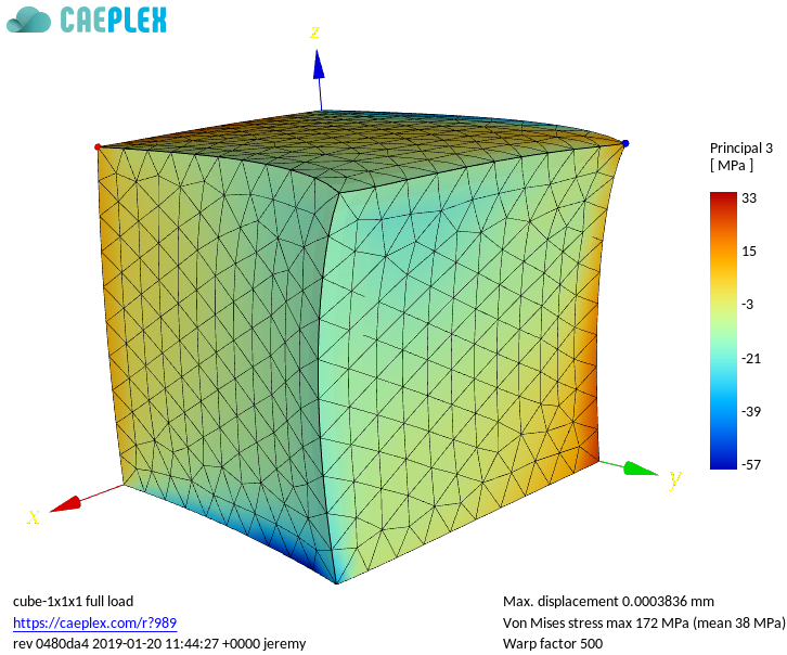{#fig:cube-full width=48%}

Spatial distribution of principal stress\ 3 for cases\ B and\ C. If linearity applied, case\ C would be equal to case\ B plus a constant :::::

In the second case, the principal stresses are not uniform and have a non-trivial distribution. Indeed, the distribution of\ $\sigma_3$ obtained by CAEplex is shown in\ [@fig:cube-shear]. Now, if we indeed were facing a fully linear problem then the results of the sum of two inputs would be equal to the sum of the individual inputs. And\ [@fig:cube-full], which shows the principal stress\ 3 of case\ C is not the result from case\ B plus any of the three constants from case\ A. Had it been, the colour distribution would be exactly the same as the scale goes automatically from the most negative value in blue to the most positive value in red. And 7+30\ $\neq$ 33. Alas, it seems that there exists some kind of unexpected non-linearity (the feared master-pet interaction?) that prevents us from from fully splitting the problem into simpler chunks.

\medskip

So what is the source of this unexpected non-linear effect in an otherwise nice and friendly linear formulation? Well, probably you already know it because after all it is almost high-school mathematics. But I learned long after college, when I had to face a real engineering problem and not just back-of-the-envelope pencil-and-paper trivial exercises.

Recall that principal stresses are the eigenvalues of the stress tensor. And the fact that in a linear elastic formulation the stress tensor of case\ C above is the sum of the individual stress tensors from cases\ A and B does not mean that their eigenvalues can be summed (think about it!). Again, imagine the eigenvalues and eigenvectors of cases A & B. Got it? Good. Now imagine the eigenvalues and eigenvectors for case\ C. Should they sum up? No, they should not! Let us make another experiment, this time with matrices using Octave or whatever other matrix-friendly program you want (try to avoid black boxes as explained in\ [@sec:two-materials]).

First, let us create a 3 $\times$ 3 random matrix $R$ and then multiply it by its transpose\ $R^T$ to obtain a symmetric matrix\ $A$ (recall that the stress tensor from [@sec:tensor] is symmetric):

octave> R = rand(3); A = R*R'
A =

   2.08711   1.40929   1.31108
   1.40929   1.32462   0.57570
   1.31108   0.57570   1.09657

Do the same to obtain another 3 $\times$ 3 symmetric matrix\ B:

octave> R = rand(3); B = R*R'
B =

   1.02619   0.73457   0.56903
   0.73457   0.53386   0.37772
   0.56903   0.37772   0.53141

Now compute the sum of the eigenvalues first and then the eigenvalues of the sum:

octave> eig(A)+eig(B)
ans =

   0.0075113
   0.8248395
   5.7674016

octave> eig(A+B)
ans =

   0.049508
   0.782990
   5.767255

Did I convince you? More or less, right? The third eigenvalue seems to fit. Let us not throw all of our beloved linearity away and dig in further into the subject. There are still two important issues to discuss which can be easily addressed using fresh-year linear algebra (remember not to fear maths!). First of all, even though principal stresses are not linear with respect to the sum they are linear with respect to pure multiplication. Once more, think what happens to the the eigenvalues and eigenvectors of a single stress tensor as all its elements are scaled up or down by a real scalar. They are the same! So, for example, the Von\ Mises stress (which is a combination of the principal stresses) of a beam loaded with a force\ $\alpha \cdot \mathbf{F}$ is\ $\alpha$ times the stress of the beam loaded with a force\ $\mathbf{F}$. Please test this hypothesis by playing with your favourite FEM solver. Or even better, take a look at the stress invariants $I_1$, $I_2$ and $I_3$ (you can search online or peek into the source code of Fino, grep for the routine called fino_compute_principal_stress()) and see (using paper and pencil!) how they scale up if the individual elements of the stress tensor are scaled by a real factor\ $\alpha$.

The other issue is that even though in general the eigenvalues of the sum of two matrices are not the same as the eigenvalues of the matrix sum, there are some cases when they are. In effect, if two matrices\ $A$ and\ $B$ commute, i.e. their product is commutative

$$ A \cdot B = B \cdot A $$ then the sums (in plural because there are three eigenvalues) of their eigenvalues are equal to the eigenvalues of the sums. In order for this to happen, both\ $A$ and\ $B$ need to be diagonalisable using the same basis. That is to say, the diagonalising matrix\ $P$ such that $P^{-1} A P$ is diagonal should be the same that renders\ $P^{-1} B P$ also diagonal. What does this mechanically mean? Well, if case\ A has loads that are somehow “independent” from the ones in case\ B, then the principal stresses of the combination might be equal to the sum of the individual principal stresses. A notable case is for example a beam that is loaded vertically in case\ A and horizontally in case\ B. I dare you to grab your FEM program one more time, run a test and picture the eigenvalues and eigenvectors of the three cases in your head.

\medskip

The moral of this fable is that if we have a case that is the combination of two other simpler cases (say one with only surface loads and one with only volumetric loads), in general we cannot just add the principal stresses (or Von Mises) of two cases and expect to obtain a correct answer. We have to solve the full case again (both the surface and the volumetric loads at the same time). In case we are stubborn enough and still want to stick to solving the cases separately, there is a trick we can resort to. Instead of summing principal stresses, what we can do is to sum either displacements or the individual stress components, which are fully linear. So we might pre-deform (or pre-stress) case B with the results from case A and then expect the FEM program to obtain the correct stresses for the combined case. However, this scheme is actually far more complex than just solving the combined case in a single run and it also needs an educated guess and/or trial and error to know at what time the pre-deformation or pre-stressing should be applied to take into account the seismic load.

ASME stress linearisation (not linearity!)

After discussing linearity, let us now dig into linearisation. The name is similar but these two animals are very different beasts. We said in\ [@sec:case] that the ASME Boiler and Pressure Vessel Code was born long before modern finite-elements methods were developed and of course being massively available for general engineering analysis (democratised?). Yet the code provides a comprehensive, sound and, more importantly, a widely and commonly-accepted body of knowledge as for the regulatory authorities to require its enforcement to nuclear plant owners. One of the main issues of the ASME code refers to what is known as “membrane” and “bending” stresses. These are defined in section\ VIII annex 5-A, although they are widely used in other sections, particularly section\ III. Briefly, they give the zeroth-order (membrane) and first-order (bending) moments (in the statistical sense) of the stress distribution along a so-called Stress Classification Line or SCL, which should be chosen depending on the type of problem under analysis.

The computation of these membrane and bending stresses are called “stress linearisation” because (I am guessing) it is like computing the Taylor expansion (or for the case, expansion in Legendre polynomials) of an arbitrary stress distribution along a line, and retaining the first two terms. That is to say, to obtain a linear approximation. More (optional) mathematical details below.

dnl figures

So what about the SCLs? Well, the ASME standard says that they are lines that go through a wall of the pipe (or vessel or pump, which is what the ASME code is for) from the inside to the outside and ought to be normal to the iso-stress curves. Stop. Picture yourself a stress field, draw the iso-stress curves (those would be the lines that have the same colour in your picture) and then imagine a set of lines that travel in a perpendicular direction to them. Finally, choose the one that seems the prettiest (which most of the time is the one that seems the easiest). There you go! You have an SCL. But there is a catch. So far, we have referred to a generic concept of “stress.” Which of the several stresses out there should you picture? One of the three normals, the three shear, Von\ Mises, Tresca? Well, actually you will have to imagine tensors instead of scalars. And there might not be such a thing as “iso-stress” curves, let alone normal directions. So pick any radial straight line through the pipe wall at a location that seems relevant and now you are done. In our case study, there will be a few different locations around the material interfaces where high stresses due to differential thermal expansion are expected to occur.

\medskip

Now the optional (but recommended) mathematical details. Accoding to ASME\ VIII Div.\ 2 Annex\ 5-A, the expression for computing the $i$-$j$-th element of the membrane tensor is

$$ \text{M}_{ij} = \frac{1}{t} \cdot \int0^t \sigma{ij}(t^\prime) \, dt^\prime $$ where $t$ is the length and $0<t^\prime<t$ is the parametrisation variable of the SCL. The other linearised stress, namely the bending stress tensor $\text{B}$ is

$$ \text{B}_{ij} = \frac{6}{t^2} \cdot \int0^t \sigma{ij}(t^\prime) \cdot \left( \frac{t}{2}-t^\prime\right) \, dt^\prime $$

For the fatigue assessment, it is the sum\ $\text{MB}$ that measures the stress

$$ \text{MB}{ij} = \text{M}{ij} \pm \text{B}_{ij} $$ where the sign should be taken such that the resulting stress intensity (i.e. Tresca, Von Mises, Principal\ 1, etc.) represents the worst-case scenario. Older versions of ASME\ VIII preferred the Tresca criterion, while newer versions switched to Von\ Mises. ASME\ III sticked to Tresca.

In any case, $\text{MB}_{ij}$ should be taken as a measure of the primary stress at the internal surface of the pipe. In effect, let us assume we have a stress distribution\ $\sigma(t^\prime)$ along a certain line of length $t$ such that\ $\sigma(0)$ and $\sigma(t)$ are the stresses at the internal and external surfaces, respectively. The primary stress distribution, i.e. the stress that is not self balancing will be of the simple linear form

$$ \sigma(t^\prime) = a\cdot t^\prime + b $$ because any other higher-order polynomial term would self-balance (exercise: prove it). The membrane and bending stresses, according to ASME would then be

$$ \text{M} = \frac{1}{t} \int{0}^{t} \big[ a\cdot t^\prime + b \big] \, dt^\prime = \frac{1}{2} \cdot a \cdot t + b $$ $$ \text{B} = \frac{6}{t^2} \int{0}^{t} \big[ a\cdot t^\prime + b \big] \cdot \left( \frac{t}{2} - t^\prime \right) \, dt^\prime = -\frac{1}{2} \cdot a \cdot t $$

In effect, we can see that $$ \sigma(0) = b = \text{M} + \text{B} $$ and

$$ \sigma(t) = a \cdot t + b = \text{M} - \text{B} $$

No need to know or even understand these integrals which for sure are not introduced to students in regular college courses. But it would be good to, as linearisation is a cornerstone subject for any serious mechanical analysis of pressurised components following the code. So get a copy of ASME sec.\ VIII div.\ 2 annex\ 5-A and then search online for for “stress linearisation” (or “linearization”).

The infinite pipe revisited after college

Let us now make a (tiny) step from the general and almost philosophical subject from the last section down to the particular case study, and reconsider the infinite pressurised pipe once again. It is time to solve the problem with a computer using finite elements and to obtain some funny coloured pictures instead of just equations.

The first thing that has to be said is that, as with any interesting problem, there are literally hundreds or different ways of solving it, each of them throwing particular conclusions. For example, one can:

1. solve a real 3D problem or a 2D axi-symmetric case (or even a 1D case using the collocation method to solve the radial dependence),
2. have a full cylindrical geometry or just a half (180º), or a quarter (90º), or a thin slice (a small amount of degrees),
3. use a structured or an unstructured grid,
4. uniformly or locally-refine the mesh (with several choices of refinement),
5. use first or second-order (or higher) elements,
6. use tetrahedra or hexahedra,
7. in the case of second-order hexahedra, use complete (i.e. 27-node hexahedron) or incomplete (i.e. 20-node hexahedron) elements,
8. have different mesh sizes from very coarse to very fine,
9. solve the same problem in a few different solvers,
10. etc.

::::: {#fig:quarter} {#fig:cube-struct width=48%}\
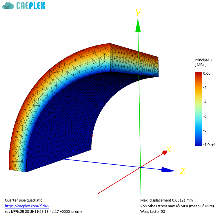{#fig:quarter-caeplex width=48%}

Two of the hundreds of different ways the infinite pressurised pipe can be solved using FEM. The axial displacement at the ends is set to zero, leading to a plane-strain condition :::::

You can get both the exponential nature of each added bullet and how easily we can add new further choices to solve a FEM problem. And each of these choices will reveal you something about the nature of either the mechanical problem or the numerical solution. It is not possible to teach any possible lesson from every outcome in college, so you will have to learn them by yourself getting your hands at them. I have already tried to address the particular case of the infinite pipe in a recent report³ that is worth reading before carrying on with this article. The conclusions of the report are:

• Engineering problems ought not to be solved using black-boxes (i.e. privative software whose source code is not freely available)---more on the subject below in\ [@sec:two-materials].
• The pressurised infinite pipe has only one independent variable (the radius $r$) and one primary dependent variable (the radial displacement $u_r$).
• The problem has analytical solution for the radial displacement\ $u_r$ and the radial\ $\sigmar$, tangential\ $\sigma\theta$ and axial\ $\sigma_z$ stresses.
• There are no shear stresses, so these three stresses are also the principal stresses.
• Analytical expressions for the membrane and membrane plus bending stresses along any radial SCL can be obtained.
• The spatial domain can be discretised using linear or higher-order elements. In particular first and second-order elements have been used in the report.
• For the same number of elements, second-order grids need more nodes than linear ones, although they can better represent curved geometries.
• The discretised problem size depends on the number of nodes and not on the number of elements---more on the subject below in\ [@sec:elements-nodes].
• The finite-element results for the displacements are similar to the analytical solution, with second-order grids giving better results for the same number of elements (this is expected as they involved far more nodes).
• The three stress distributions computed with the finite-element give far more reasonable results for the second-order case than for the first-order grid. This is qualitatively explained by the fact that first-order tetrahedra have uniform derivatives and such the elements located in both the external and external faces represent the stresses not at the actual faces but at the barycentre of the elements.
• Membrane stresses converge well for both the first and second-order cases because they represent a zeroth-order moment of the stress distribution and the excess and defect errors committed by the internal and external elements approximately cancel out.
• Membrane plus bending stresses converge very poorly with linear elements because the excess and defect errors do not cancel out because it is a first-order moment of the stress distribution.
• The computational effort to solve a given problem, namely the CPU time and the needed RAM ([@fig:error-vs-cpu]) depend non-linearly on various factors, but the most important one is the problem size which is three times the number of nodes in the grid---more on the subject below in\ [@sec:elements-nodes].
• The error with respect to the analytical solutions as a function of the CPU time needed to compute the membrane stress is similar for both first and second-order grids. But for the computation of the membrane plus bending stress ([@fig:error-MB-vs-cpu]), first-order grids give very poor results compared to second-order grids for the same CPU time.

::::: {#fig:error-vs-cpu} {#fig:error-M-vs-cpu width=90%}

{#fig:error-MB-vs-cpu width=90%}

Error in the computation of the linearised stresses vs. CPU time needed to solve the infinite pipe problem using the finite element method :::::

An additional note should be added. The FEM solution, which not only gives the nodal displacements but also a method to interpolate these values inside the elements, does not fully satisfy the original equilibrium equations at every point (i.e. the strong formulation). It is an approximation to the solution of the weak formulation that is close (measured in the vector space spanned by the shape functions) to the real solution. Mechanically, this means that the FEM solution leads only to nodal equilibrium but not pointwise equilibrium.

Elements, nodes and CPU

The last two bullets above lead to an issue that has come many times when discussing the issue of convergence with respect to the mesh size with other colleagues. There apparently exists a common misunderstanding that the number of elements is the main parameter that defines how complex a FEM model is. This is strange, because even in college we are taught that the most important parameter is the size of the stiffness matrix, which is three times (for 3D problems with the displacement-based formulation formulation) the number of nodes.

Let us pretend we are given the task of comparing two different FEM programs. So we solve the same problem in each one and see what the results are. I have seen many times the following situation: the user loads the same geometry in both programs, run the meshing step in both of them so that the number of elements is more or less them same (because she wants to be “fair”) and then solves the problem. Voilà! It turns out that the first program defaults to first-order elements and the second one to second-order elements. So if the first one takes one minute to obtain a solution, the second one should take nearly four minutes. How come that is a fair comparison? Or it might be the case that one program uses tetrahedra while the other one defaults to hexahedra. Or any other combination. In general, there is no single problem parameter that can be fixed to have a “fair” comparison, but if there was, it would definitely be the number of nodes rather than the number of elements. Let us see why.

\medskip

Fire up your imagination again and make a thought experiment in which you have to compare say a traditional FEM approach with a new radical formulation that a crazy mathematician from central Asia came up with claiming it is a far superior theory than our beloved finite elements (or for the case, any other formulation from\ [@sec:formulations]). How can we tell if the guy is really a genius or purely nuts? Well, we could solve a problem which we can compute the analytical solution (for example the infinite pipe from\ [@sec:infinite-pipe]) first with the traditional method ([@sec:infinite-pipe-fem]) and then with the program which uses the new formulation. Say the traditional FEM gives an error between 1% and 5% running in a few seconds depending on the mesh size. The new program from the crazy guy takes no input parameters and gives an error of 0.1%, but it takes one week of computation to produce a result. Would you say that the new radical formulation is really far superior?

What I would do is to run a FEM program that takes also one week to compute, and only then compare the errors. So that is why\ [@fig:error-vs-cpu] uses the CPU time in the abscissas rather than the number of elements to compare first and second-order formulations.

To fix ideas, let us stick to a linear elastic FEM problem. The CPU time needed to completely solve such a problem can be divided into four steps:

1. meshing the continuous geometry,
2. building the stiffness matrix,
3. solving the equations to obtain the displacements, and
4. computing the stress from the displacements.

Meshing

The effort needed to compute a discretisation of a continuous domain depends on the meshing algorithm. But nearly all meshers first put nodes on the edges (1D), then on the surfaces (2D) and finally on the volumes (3D). Afterwards, they join the nodes to create the elements. Depending on the topology (i.e. tetrahedra, hexahedra, pyramids, etc) and the order (i.e. linear, quadratic, etc.) this last step will vary, but the main driver here is the number of nodes. Try measuring the time needed to obtain grids of different sizes and kinds with your mesher.

Building

The stiffness matrix is a square matrix that has\ $NG$ rows and\ $NG$ columns where $N$ is the number of nodes and $G$ is the number of degrees of freedom per node, which for three-dimensional problems is $G=3$. But even though FEM problems have to build a $NG\times NG$ matrix, they usually sweep through elements rather than through nodes, and then scatter the elements of the elemental matrices to the global stiffness matrix. This is called the assembly of the matrix. So the effort needed here depends again on how the solver is programmed, but it is a combination of the number of elements and the number of nodes.

For a fixed number of nodes, first-order grids have far more elements than second-order grids because in the first case each node has to be a vertex while in the latter half will be vertexes and half will be located at the edges (think!). So the sweep is larger for linear grids. But the effort needed to integrate quadratic shape functions is greater than for the linear case, so these two effects almost cancel out.

Solving

The linear FEM problem leads of course of a system of\ $NG$ linear equations, cast in matrix form by the stiffness matrix\ $K$ and a right-hand size vector\ $\mathbf{b}$ containing the loads (both volumetric and the ones at the surfaces from the boundary conditions):

$$K \cdot \mathbf{u} = \mathbf{b}$${#eq:kub}

The objective of the solver is to find the vector\ $\mathbf{u}$ of nodal displacements that satisfy the momentum equilibrium. Luckily (well, not purely by chance but by design) the stiffness matrix is almost empty. It is called a sparse matrix because most of its elements are zero. If it was fully filled, then a problem with just 100k nodes would need more than 700\ Gb of RAM just to store the matrix elements, rendering FEM as practically impossible. And even though the stiffness matrix is sparse, its inverse is not so we cannot solve the elastic problem by “inverting” the matrix. Particular methods to represent and more importantly to solve linear systems involving these kind of matrices have been developed, which are the methods used by finite-element (and the other finite-cousins) programs. In general there are two approaches

• direct, where a rather complex algorithm for building partial decompositions (LU, QR, Cholesky, etc.) are used in order to avoid needing aforementioned the 700\ Gb of RAM, or
• iterative, meaning that at each step of the iteration the numerical answer improves, i.e. $\left|K \cdot \mathbf{u} - \mathbf{b}\right| \rightarrow 0$. Even though in particular for Krylov-subspace methods, $K \cdot \mathbf{u} - \mathbf{b} = \mathbf{0}$ after\ $NG$ steps, a few dozen of iterations are usually enough to assume that the problem is effectively solved (i.e. the residual is less than a certain threshold).

So the question is… how hard is to solve a sparse linear problem? Well, the number of iterations and the complexity of the partial decompositions needed to attain convergence depends on the spectral radius of the stiffness matrix\ $K$, which in turns depend on the elements themselves, which depend mainly on the parameters of the elastic problem. But it also depends on how sparse\ $K$ is, which changes with the element topology and order. [@Fig:test] shows the structure of two stiffness matrices for the same linear elastic problem discretised using exactly the same number of nodes but using linear and quadratic elements respectively. The matrices have the same size (because the number of nodes is the same) but the former is more sparse than the latter. Hence, it would be harder (in computational terms of CPU and RAM) to solve the second-order case.

::::: {#fig:test} {#fig:test1 width=48%}\
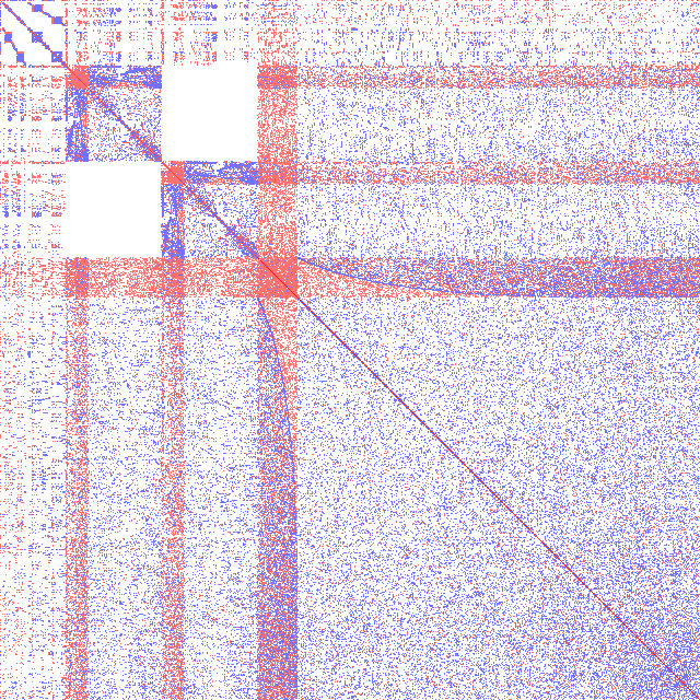{#fig:test2 width=48%}

Structure of the stiffness matrices for the same FEM problem with 10k nodes. Red (blue) are positive (negative) elements :::::

In a similar way, different types of elements will give rise to different sparsity patterns which change the effort needed to solve the problem. In any case, the base parameter that controls the problem size and thus provides a basic indicator of the level of difficulty the problem poses is the number of nodes. Again, not the number of elements, as the solver does not even know if the matrix comes from FEM, FVM or FDM.

Stress computation

In the displacement-based formulation, the solver finds the displacements\ $\mathbf{u}(\mathbf{x})$ that satisfy [@eq:kub], which are the principal unknowns. But from\ [@sec:tensor] we know that we actually have solved the problem after we have the stress tensors at every location\ $\mathbf{x}$, which are the secondary unknowns. So the FEM program has to compute the stresses out of the displacements. It first computes the strain tensor, which is composed of the nine partial derivatives of the three displacements with respect to the three coordinates. Then it computes the stress tensor (atready introduced in\ [@sec:tensor]) using the materials’ strain-stress constitutive equations which involve the Young Modulus\ $E$, the Poisson ratio\ $\nu$ and the spatial derivatives of the displacements\ $\mathbf{u}=[u,v,w]$. This sounds easy, as we (well, the solver) knows what the shape functions are for each element and then it is a matter of computing nine derivatives and multiplying by something involving\ $E$ and\ $\nu$. Yes, but there is a catch. As the displacements\ $u$, $v$ and\ $w$ are computed at the nodes, we would like to also have the stresses at the nodes. However,

i. the displacements\ $\mathbf{u}(\mathbf{x})$ are not differentiable at the nodes, and ii. if the node belongs to a material interface, neither\ $E$ nor\ $\nu$ are defined.

Let us focus on the first item and leave the second one for a separate discussion in\ [@sec:two-materials]. The finite-element method computes the principal unknowns at the nodes and then says “interpolate the nodal values inside each element using its shape functions.” It sounds (and it is) great, but a node belongs to more than one element (you can now imagine a 3D mesh composed of tetrahedra but you can also simplify your mind pictures by thinking in just one dimension: a node is shared by two segments). So the slope of the interpolation when we move from the node into one element might (and it never is) the same as when we move from the same node into another element. Stop and think. Now let us take a look at [@fig:derivatives]. It shows four finite-element solutions for a certain problem that has a cosine as the analytical solution. All the cases use eight elements: either uniformly distributed along the domain $x \in [-1:+1]$ or only one element in the negative half and the remaining seven evenly distributed between zero and one, configuring a rather extreme non-uniform grid to better illustrate the point. Both first and second-order elements were used for each mesh, hence obtaining four combinations. We know the derivative of the analytical solution is zero at $x=0$. In the uniform cases of [@fig:slab-1-0;@fig:slab-2-0], if we took the average of the derivatives at each side of the origin we would obtain zero as expected. But in the non-uniform cases\ [@fig:slab-1-1;@fig:slab-2-1], plain averaging fails even in the quadratic case.

::::: {#fig:derivatives} {#fig:slab-1-0 width=48%}\
{#fig:slab-1-1 width=48%}

{#fig:slab-2-0 width=48%}\
{#fig:slab-2-1 width=48%}

Solution of a problem using FEM using eight linear/quadratic uniform/non-uniform elements. The reference solution is a cosine. Plain averaging works for uniform grids but fails in the non-uniform cases. :::::

Now proceed to picturing the general three-dimensional cases with unstructured tetrahedra. What is the derivative of the displacement\ $v$ in the\ $y$ direction with respect to the $z$ coordinate at a certain node shared by many tetrahedra? What if one of the elements is very small? Or it has a very bad quality (i.e. it is deformed in one direction) and its derivatives cannot be trusted? Should we still average? Should this average be weighted? How?

Detailed mathematics show that the location where the derivatives of the interpolated displacements are closer to the real (i.e. the analytical ones in problems that have it) solution are the elements’ Gauss points. Even better, the material properties at these points are continuous (they are usually uniform but they can depend on temperature for example) because, unless we are using weird elements, there are no material interfaces inside elements. But how to manage a set of stresses given at the Gauss points instead of at the nodes? Should we use one mesh for the input and another one for the output? What happens when we need to know the stresses on a surface and not just in the bulk of the solid? There are still no one-size-fits-all answers. There is a very interesting blog post by Nick Stevens that addresses the issue of stresses computed at sharp corners. What does your favourite FEM program do with such a case?

In any case, this step takes a non-negligible amount of time. The most-common approach, i.e. the node-averaging method is driven mainly by the number of nodes of course. So all-in-all, these are the reasons to use the number of nodes instead of the numbers of elements as a basic parameter to measure the complexity of a FEM problem.

Adding complexity: the truth is out there

Let us review some issues that appear when solving our case study and that might not have been thoroughly addressed back during our college days.

Two (or more) materials

The main issue with fatigue in nuclear piping during operational transients is that at the welds between two materials with different thermal expansion coefficients there can appear potentially-high stresses during temperature changes. If these transients are repeated cyclically, fatigue may occur. We already have risen a warning flag about stresses at material interfaces in\ [@sec:two-materials]. Besides all the open questions about computing stresses at nodes, this case also adds the fact that the material properties (say the Young Modulus\ $E$) is different in the elements that are at each side of the interface.

::::: {#fig:two-cubes} {#fig:two-cubes2 width=48%}\
{#fig:two-cubes4 width=48%}

Two cubes of different materials (the one in the left soft, the one in the right hard) share a face and a pressure is applied at the right-most face :::::

To simplify the discussion that follows, let us replace for one moment the full $3 \times 3$ tensor and the nine partial derivatives of the displacement by just one strain\ $\epsilon$ and let the linear elastic strain-stress relationship to be the simple scalar expression

$$ \sigma = E \cdot \epsilon $$

Faced with the problem of computing the stress\ $\sigma$ at one node shared by many elements, we might:

1. compute the (weighted?) averages\ $\langle E \rangle$ and $\langle \epsilon \rangle$ and then compute the stress as

   $$ \langle \sigma \rangle = \langle E \rangle \cdot \langle \epsilon \rangle$$

   This would be like having a meta-material at the interface with average properties, or

2. compute the stress as the (weighted?) average of the product $E \cdot \epsilon$ in each node

   $$ \langle \sigma \rangle = \langle E \cdot \epsilon \rangle$$

   This would be like forcing a non-differentiable function to behave smoothly, or

3. internally duplicate the nodes at the interface and compute one stress for each material. This would result in a stress distribution which is not a real function because the same location\ $\mathbf{x}$ will be associated to more than one stress value, or

4. duplicate the surface elements at the interfaces and solve the problem using a contact formulation. This would render the problem non-linear and add the complexity of having to find appropriate penalty coefficients.

There might be other choices as well. Do you know what your favourite FEM program does? Now follow up with these questions:

a. Does the manual say? b. Does it tell you the details like how it weights the averages? c. Does it discard values that are beyond a number of standard deviations away? d. How many standard deviations? e. …

You can still add a lot of questions that you should be having right now. If you cannot get a clear answer for at least one of them, then start to worry. After you do, add the following question:

Do you believe your favourite FEM program’s manual?

What we as responsible engineers who have to sign a report stating that a nuclear power plant will not collapse due to fatigue in its pipes, is to fully understand what is going on with our stresses. Richard Stallman says that the best way to solve a problem is to avoid it in the first place. In this case, we should avoid having to trust a written manual and rely on software whose source code is available. What we need is the capacity (RMS calls it freedom) to be able to see the detailed steps performed by the program so we can answer any question we (or other people) might have.

Without resorting into philosophical digressions about the difference between free and open-source software (not because it is not worth it, but because it would take a whole book), the programs that make their source code available for their users are called open-source software. If the users can also modify and re-distribute the modified versions, they are called free software. Note that the important concept here is freedom, not price. In Spanish (my native language) it would have been easier because there are two separate words for free as in freedom (“libre”) and for free as in price (“gratis”).

In effect, a couple of years ago Angus Ramsay noted a weird behaviour in the results given by a certain commercial non-free FEA software regarding the handling of expansion coefficients from ASME data. To understand what was going on, Angus and I had to guess what the program was doing to reproduce the allegedly weird results. Finally, it was a matter how the data was rounded up to be presented in a paper table rather than a programming flaw. Nevertheless, we were lucky our guesses lead us to a reasonable answer. If we had access to the program’s source code, we could have thoroughly analysed the issue in a more efficient way. Sure, we might not have the same programming skills the original authors of the software have, but if it had been free software we would have had the freedom to hire a programmer to help us out. That is what free means. In Eric Raymond’s words, “given enough eyeballs, all bugs are shallow.” This is rather important in engineering software where verification and validation is a must, especially in regulated fields like the nuclear industry. First, think how can a piece of software be verified if the source code is not available for independent analysis. And then, ask yourself another question:

Do you trust your favourite FEM program?

Back to the two-material problem, all the discussion above in\ [@sec:two-materials] about non-continuous derivatives applies to a sharp abrupt interface. In the study case the junctions are welded so there is a heat-affected zone with changes in the material micro structure. Therefore, there exists a smooth transition from the mechanical properties of one material to the other one in a way that is very hard to predict and to model. In principle, the assumption of a sharp interface is conservative (in the sense of\ [@sec:kinds]). There cannot be an SCL exactly on a material interface so there should be at least two SCLs, one at each side of the junctions of\ [@fig:weldolet-scls;@fig:valve-scls1] illustrate. The actual distance would have to be determined first as an educated guess, then via trial and error and finally in accordance with the regulator.

A parametric tee

Time for another experiment. We know (more or less) what to expect from an infinite pressurised pipe from\ [@sec:infinite-pipe] and [@sec:infinite-pipe-fem]. What if we added a branch to such pipe? Even more, what if we successively varied the diameter of the branch to see what happens? This is called parametric analysis, and sooner or later (if not now) you will find yourself performing this kind of computations more often than any other one.

So here come the five Feynmann-Ohno questions:

1. Why do you want to perform a parametric computation?
   So we can study how the linearised stresses change with the inclusion of a branch of a certain diameter (and because we can, using the PARAMETRIC keyword in Fino).

2. Why do you want to know how the stresses change with the inclusion of a branch?
   Because, if we have the time, it is worth to do something harder than originally asked (football joke: it is like training throw-ins with watermelons during the week so you can reach the area with a regular ball on the weekends).

3. Why do you want to do something harder?
   Because getting out of our comfort zone once in a while is a healthy habit.

4. Why is getting out of our comfort zone a healthy habit?
   Because it fires up a certain part of our brains that keep us active and allow us to better understand what is it that is going on with the problem we are solving.

5. Why do you want to understand what is going on?
   For the same reason you are now reading this chapter.

Let us solve the following mock-up case: a long main 12-inch schedule\ 80 pipe has an orthogonal branch of a certain nominal diameter of\ $d_b$\ inches (it seems that the SI did not do well amongst the piping engineering community). Both the main line and the branch are pressurised with\ $p=10$\ MPa. The main pipe is aligned with the\ $x$ axis and the branch coincides with the\ $z$ axis. Thus, the $x$-$z$ plane acts as a symmetry plane and we only need to model two octants of the full geometry, as shown in\ [@fig:tee-geo]. Note that the tee is modelled as the boolean intersection of two cylinders. There are no filleted edges nor rounded corners or any other smoothing. A real CAD file containing the appropriate geometry needs to be built for the real case study.

::::: {#fig:tee-geo} {#fig:tee-geo1 width=54%}\
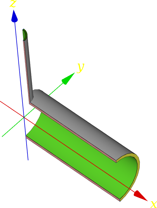{#fig:tee-geo2 width=44%}

Geometry of the parametric 12-inch tee for the particular case of a 4-inch branch :::::

The boundary conditions are

• Magenta: axial symmetry $u=0$
• Salmon: plane symmetry $v=0$
• Yellow: axial $u=0$ and radial symmetry $0=vz-wy$
• Dark green: axial $w=0$ and radial symmetry $0=vx-uy$
• Light green: internal pressure\ $p=10$\ MPa

Three radial SCLs---namely cyan, yellow and green---are located at a distance of one thickness of the main line from the external wall of the branch into the main direction\ $x$ ([@fig:tee-scls]). In\ [@fig:tee-MB] we can see the results of the parametric computation, namely the linearised membrane and bending stresses computed in each of the three SCLs as a function of\ $d_b$. Note that\ $d_b$ is a continuous variable and even unreal values (such as 9-inches) were used to perform the parametric run. The thickness of such cases was interpolated using actual schedule-80 geometrical data from ASME\ B36.310M.

::::: {#fig:tee-scls} {#fig:tee-scls1 width=29%}\
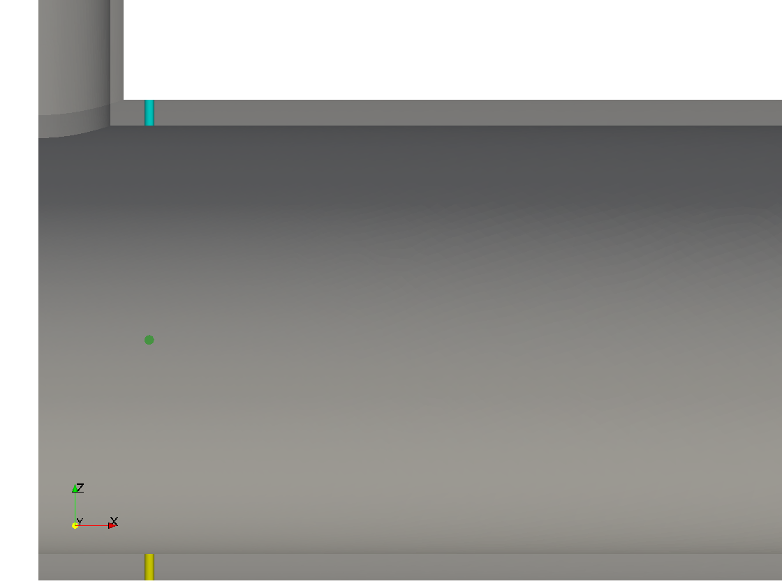{#fig:tee-scls2 width=67%}

:::::

:::::

:::::

:::::

:::::

:::::

:::::

:::::

:::::

::::: {#fig:tee-MB} {#fig:M width=90%}

{#fig:B width=90%}

Parametric membrane and bending stresses as a function of the nominal diameter\ $d_b$ of the branch :::::

::::: {#fig:tee-post} {#fig:tee-post-2 width=30%}\
{#fig:tee-post-5 width=30%}\
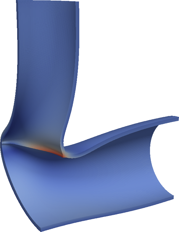{#fig:tee-post-10 width=30%}

Von\ Mises stress and 400x warped displacements for three values of\ $d_b$ :::::

[@Fig:tee-post] illustrates how the pipes deform when subject to the internal pressure. When the branch is small, the problem resembles the infinite-pipe problem where the main pipe expands radially outward and there is only traction. For large values of\ $d_b$, the pressure in the branch bends down the main pipe, generating a complex mixture of traction and compression. The tipping point seems to be around a branch diameter\ $d_b\approx 5$\ in.

Do you now see the added value of training throw-ins with watermelons? We might go on…

• studying how the maximum Von\ Mises stress as a function the radius\ $r_f$ of an hypothetical fillet operation on the tee’s sharp edges,
• making the branch another material and adding thermal expansion,
• adding piping supports to restrain the degrees of freedom of the pipes,
• using distributed forces from earthquakes,
• etc.

Most of the time at college we would barely do what is needed to be approved in one course and move on to the next one. If you have the time and consider a career related to finite-element analysis, please do not. Clone the repository⁴ with the input files for Fino and start playing. If you are stuck, do not hesitate asking for help in wasora’s mailing list.

One further detail: it is always a sane check to try to explain the numerical results based on physical reasoning (i.e. “with your fingers”) as we did two paragraphs above. Most of the time you will be solving problems whilst already knowing what the result would (or ought to) be.

Bake, shake and break

A fellow mechanical engineer who went to the same high school I did, who went to the same engineering school I did and who worked at the same company I did, but who earned a PhD in Norway once told me two interesting things about finite-elements graduate courses. First, that in Trondheim the classes were taught by faculty from the the mathematics department rather than from the mechanical engineering department. It made complete sense to me, as I always have thought finite elements mainly as a maths subject. And even though engineers might know some maths, it is nothing compared to actual mathematicians. Secondly, that they called the thermal, natural oscillations and elastic problems as the rhyming trio “bake, shake and break” (they also had “wake” for fluids, but that is a different story). These are just the three problems listed in section\ [@sec:piping-nuclear] that we need to solve in our nuclear power plant.

So here we are again with the case study where we have to compute the linearised stresses at certain SCLs located near the interface between two different kinds of steels during operational and incidental transients of the plant. The first part is then to “bake” the pipes, modelling a thermal transient with time-dependent temperature or convection boundary conditions (it depends on the system). This steps gives a time and space-dependent temperature\ $T(x,y,z,t)$.

Then we proceed to “shake” the pipes, i.e. to compute the natural frequencies and associated oscillations modes. Employing the floor response spectra and combining the individual contributions with the SRSS method discussed in section\ [@sec:seismic], we obtain a distributed load vector\ $\mathbf{f}(x,y,z)$ which is statically equivalent to the design earthquake.

Finally we attempt to “break” the pipes successively solving many steady-state elastic problems for different times\ $t$ of the operational transient. Some remarks about this step:

1. The material properties are temperature-dependent (we use data from ASME\ II part\ D).
2. Thermal expansion is taken into account. The reference temperature (i.e. the temperature at which there is no expansion) is\ 20ºC that coincides with ASME’s decision of the reference temperature for the mean thermal expansion coefficients.
3. The temperature distribution\ $T(x,y,t,z)$ for bullets 1 & 2 is the generalisation of the reduced-model procedure explained in\ [@sec:thermal].
4. The internal faces of the pipes are subject to an uniform pressure\ $p(t)$ given by the definition of the transient.
5. There are mechanical supports throughout the piping system. Depending on the type of the support (i.e. vertical, lateral, axial, full, etc.) one or more degrees of freedom (i.e. $u$, $v$ and/or $w$) are fixed to zero. The ends of the CAD models are chosen always to have axially-null displacements.
6. The earthquake-equivalent volumetric force\ $\mathbf{f}(x,y,z)$ is only be applied at the time\ $t$ where the maximum stresses occur. Note that due to the discussion from\ [@sec:linearity] we cannot compute the stresses raised just by\ $\mathbf{f}(x,y,z)$ and then add them to the main stresses. The force has to be included into the “break” step. An educated guess of the time where the maximum stress occur is usually enough. Anyway, it might be necessary a trial and error scheme to find the sweet spot.
7. According to ASME\ III, the seismic load has to be applied during two seconds with the two possible signs. That is to say, apply $\mathbf{f}(x,y,z)$ during two seconds and then $-\mathbf{f}(x,y,z)$ during two further seconds when the main stresses are maximums.
8. A number of stress classification lines have to be defined. The locations should be previously accorded with the plant owner and/or the regulator.
9. The stress linearisation has to be performed individually for each principal stress\ $\sigma_1$, $\sigma_2$ and $\sigma_3$ to fulfil the requirements ASME\ III\ NB-3126 (see [@sec:in-air] below).
   
10. This “break” step is linear.

Is the last bullet right? Surely you’re joking, Mr.\ Theler! Linear problems are simple and almost useless. How can this extremely complex problem be linear? Well, let us see. First, there are two main kinds of non-linearities in FEM:

1. Geometrical non-linearities
2. Material non-linearities

The first one is easy. Due to the fact that the pipes are made of steel, it is expected that the actual deformations are relatively small compared to the original dimensions. This leads to the fact that the mechanical rigidity (i.e. the stiffness matrix) does not change significantly when the loads are applied. Therefore, we can safely assume that the problem is geometrically linear.

Let us now address material non-linearities. On the one hand we have the temperature-dependent issue. According to ASME\ II part\ D, what depends on temperature\ $T$ is the Young Modulus\ $E$. But the stress-strain relationship is yet

$$ \sigma = E(T) \cdot \epsilon $$

What changes with temperature is the slope of\ $\sigma$ with respect to\ $\epsilon$ (think and imagine!), but the relationship between them is still linear.

On the other hand, we have a given non-trivial temperature distribution\ $T(\mathbf{x}, t)$ within the pipes that is a snapshot of a transient heat conduction problem at a certain time\ $t$ (think and picture yourself taking photos of the temperature distribution changing in time). Let us now forget about the time, as after all we are solving a steady-state elastic problem. Now you can trust me or ask a FEM teacher, but the continuous displacement formulation can be loosely written as

$$ K\big[E\left(T(\mathbf{x})\right), \mathbf{x}\big] \cdot \mathbf{u}(\mathbf{x}) = \mathbf{b}(\mathbf{x})$$

If you notice, the complex dependence of the stiffness matrix\ $K$ can be reduced to just the spatial vector\ $\mathbf{x}$:

$$ K(\mathbf{x}) \cdot \mathbf{u}(\mathbf{x}) = \mathbf{b}(\mathbf{x})$$

And this last equation is linear in\ $\mathbf{u}$. In effect, the discretisation step means to integrate over\ $\mathbf{x}$. As\ $K$, $\mathbf{u}$ and\ $\mathbf{b}$ depend only on\ $\mathbf{x}$, then after integration one gets just numbers with the matrix representation of\ [@eq:kub]. Again, you can either trust me, ask a teacher or go through with the maths (in increasing order of recommendation).

::::: {#fig:case-cad} 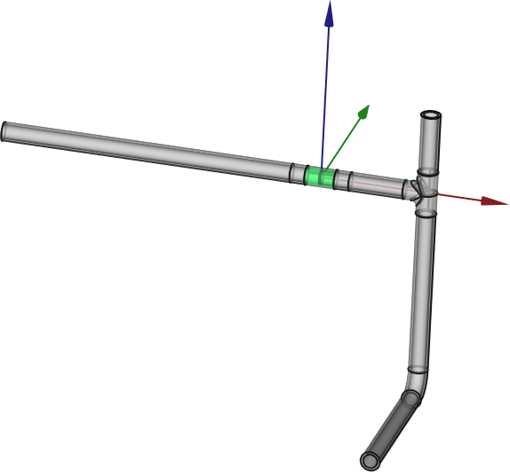{#fig:case-cad1 width=75%}

{#fig:case-cad2 width=95%}

:::::

:::::

:::::

:::::

:::::

:::::

:::::

:::::

:::::

:::::

:::::

:::::

:::::

:

::::: {#fig:case-mesh} {#fig:case-mesh1 width=85%}

{#fig:case-mesh2 width=100%}

Unstructured grid for the mechanical analysis. Volumetric elements (i.e. tetrahedra) corresponding to carbon steel are magenta and to stainless steel are green. Surface elements (i.e. triangles) corresponding to the internal pressurised face are yellow :::::

{#fig:case-scls width=75%}

::::: {#fig:case-temp} {#fig:case-temp1 width=70%}

{#fig:case-temp2 width=100%}

:::::

:::::

:::::

:::::

:::::

:::::

:::::

:::::

:::::

:::::

:::::

:::::

:::::

:::::

:::::

:::::

:::::

:::::

:::::

:::::

:::::

:::::

:::::

:::::

:::::

:::::

:::::

:::::

:::::

:::::

:::::

:::::

:::::

:

::::: {#fig:case-mode} {#fig:case-mode-1 width=30%}\
{#fig:case-mode-2 width=30%}\
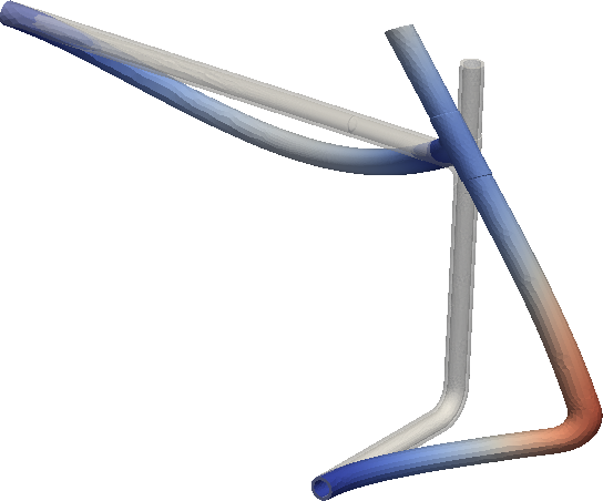{#fig:case-mode-3 width=30%}

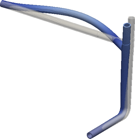{#fig:case-mode-4 width=30%}\
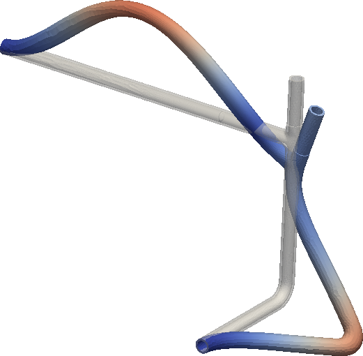{#fig:case-mode-5 width=30%}\
{#fig:case-mode-6 width=30%}

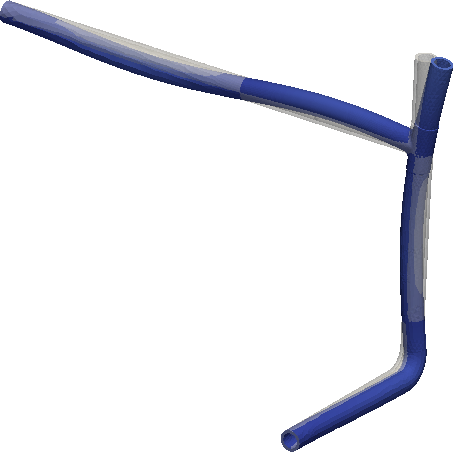{#fig:case-mode-7 width=30%}\
{#fig:case-mode-8 width=30%}\
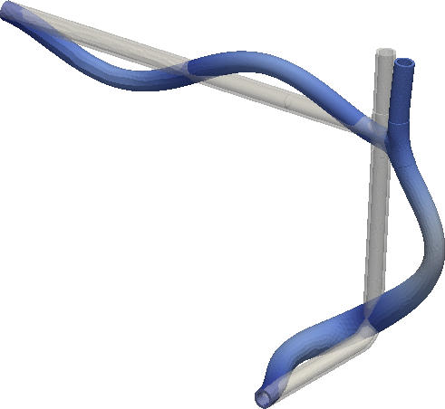{#fig:case-mode-9 width=30%}

First nine natural modes of oscillation of the piping system subject to the boundary conditions the supports provide :::::

{#fig:case-spectrum width=80%}

::::: {#fig:case-acceleration} {width=50%}

{width=50%}

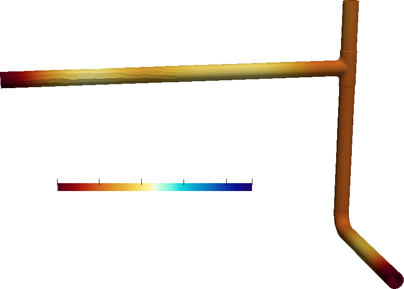{width=50%}

The static equivalent accelerations for the spectra of\ [@fig:case-spectrum] computed using the SRSS method :::::

\medskip

To recapitulate, the figures in this section show some partial non-dimensional results of an actual system of a certain nuclear power plant. The main issues to study were the interfaces between a carbon-steel pipe and a stainless-steel orifice plate used to measure the (heavy) water flow through the line. The steps discussed so far include

1. building a CAD model of the piping section under study, which will be the main domain ([@fig:case-cad] or [@fig:real-life;@fig:weldolet-cad;@fig:valve-cad1])
2. creating a mesh for the main domain refining locally around the material interfaces ([@fig:case-mesh] or [@fig:weldolet-mesh;@fig:valve-mesh1;@fig:real-mesh2])
3. defining the number and locations of the SCLs ([@fig:case-scls] or [@fig:weldolet-scls;@fig:valve-scls1;@fig:tee-scls])
4. computing a heat conduction (bake) transient problem with temperatures as a function of time from the operational transient in a simple domain using temperature-dependent thermal conduction coefficients from ASME\ II\ part D ([@fig:case-temp] or [@fig:valve-temp;@fig:real-mesh2])
5. generalising the temperature distribution as a function of time to the general domain ([@fig:case-temp2] or [@fig:valve-gen;@fig:real-gen])
6. performing a modal analysis (shake) on the main domain to obtain the main oscillation frequencies and modes ([@fig:case-mode] or [@fig:modes])
7. using the floor response spectra ([@fig:case-spectrum] or [@fig:spectrum]) and the SRSS method to obtain a distributed force statically-equivalent to the earthquake load ([@fig:case-acceleration] or [@fig:acceleration])
8. successively solving the linear elastic problem for different times using the generalised temperature distribution taking into account a. the dependence of the Young Modulus\ $E$ and the thermal expansion coefficient\ $\alpha$ with temperature, b. the thermal expansion effect itself c. the instantaneous pressure exerted in the internal faces of the pipes at the time\ $t$ according to the definition of the operational transient d. the restriction of the degrees of freedom of those faces, lines or points that correspond to mechanical supports located both within and at the ends of the CAD model e. the earthquake load, which according to ASME should be present only during four seconds of the transient: two seconds with one sign and the other two seconds with the opposite sing. This period should be selected to coincide with the instant of highest mechanical stress (conservative computation)
9. computing the linearised stresses (membrane and membrane plus bending) at the SCLs combining them as a. Principal 1 b. Principal 2 c. Principal 3 d. Tresca
10. juxtaposing these linearised stresses for each time of the transient and for each transient so as to obtain a single time-history of stresses including all the operational and/or incidental transients under study, which is what stress-based fatigue assessment needs (recall\ [@sec:fatigue] and go on to\ [@sec:usage]).

A pretty nice list of steps, which definitely I would not have been able to tackle when I was in college. Would you?

Cumulative usage factors

Strictly speaking, finite elements are not needed anymore at this point of the analysis. But even though we are (or want to be) FEM experts, we have to understand that if the objective of a work is to evaluate fatigue (or fracture mechanics or whatever), finite elements are just a mean and not and end. If we just mastered FEM and nothing else, our field of work would be highly reduced. We need to use all of our computational knowledge to perform actually engineering tasks and to be able to tell our bosses and clients whether the pipe would fail or not. This tip is induced in college but it is definitely reinforced afterwards when working with actual clients and bosses.

Another comment I would like to add is that I had to learn fatigue practically from scratch when faced with this problem for the first time in my engineering career. I remembered some basics from college (like the general introduction from [@sec:fatigue]), but I lacked the skills to perform a real computation by myself. Luckily there still exist books, there are a lot of interesting online resources (not to mention Wikipedia) and, even more luckily, there are plenty of other fellow engineers that are more than eager to help you. My second tip is: when faced to a new challenging problem, read, learn and ask for guidance to real people to see if you read and learned it right.

\medskip

Back and distantly, in\ [@sec:case] we said that people noticed there were some environmental factors that affected the fatigue resistance of materials. The basic ASME approach does not take care of these factors, and it is regarded as fatigue “in air.” We are interested in taking them into account, so we follow the US Nuclear Regulatory Commission guidelines to evaluate fatigue “in water.”

In air (ASME’s basic approach)

We already said in\ [@sec:fatigue] that the stress-life fatigue assessment method gives the limit number\ $N$ of cycles that a certain mechanical part can withstand when subject to a certain periodic load of stress amplitude\ $S\text{alt}$. If the actual number of cycles\ $n$ the load is applied is smaller than the limit\ $N$, then the part is fatigue-resistant. In our case study there is a mixture of several periodic loads, each one expected to occur a certain number of times. ASME’s way to evaluate the resistance is to break up the stress history into partial stress amplitudes\ $S{\text{alt},j}$ between a “peak” and a “valley” and to compute individual usage factors\ $U_j$ for the\ $j$-th amplitude (which does not need to coincide with one of the \ $k$ transient loads) as

$$U_j = \frac{n_j}{N_j}$$

The overall cumulative usage factor is then the algebraic sum of the partial contributions

$$\text{CUF} = U_1 + U_2 + \dots + U_j + \dots$$

If\ $\text{CUF} < 1$, then the part under analysis can withstand the proposed cyclic operation.

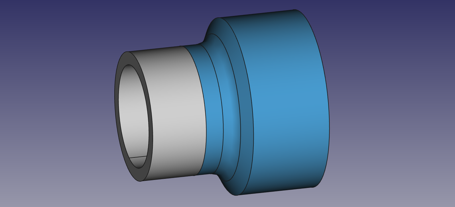{#fig:axi-inches-3d width=80%}

If the extrema of the partial stress amplitude correspond to different transients, then the following note in ASME III’s NB-3224(5) should be followed:

In determining $n_1$, $n_2$, $n_3$, $\dots$, $n_j$ consideration shall be given to the superposition of cycles of various origins which produce a total stress difference range greater than the stress difference ranges of the individual cycles. For example, if one type of stress cycle produces 1,000 cycles of a stress difference variation from zero to +60,000\ psi and another type of stress cycle produces 10,000 cycles of a stress difference variation from zero to −50,000\ psi, the two types of cycle to be considered are defined by the following parameters:

(a) for type 1 cycle, $n1 =$ 1,000 and $S{\text{alt},1} = (60,000 + 50,000)/2 = 55,000$\ psi; (b) for type 2 cycle, $n2 =$ 9,000 and $S{\text{alt},2} = (50,000 + 0)/2 = 25,000$\ psi.

This cryptic paragraph can be better explained by using a clearer example. To avoid using actual sensitive data from a real power plant, let us use the same test case used by both the US Nuclear Regulatory Commission (in its report NUREG/CR-6909) and the Electric Power Institute (report 1025823) called “EAF (Environmentally-Assisted Fatigue) Sample Problem 2-Rev.\ 2 (10/21/2011)”.

It consists of a typical vessel (NB-3200) nozzle with attached piping (NB-3600) as illustrated in\ [@fig:axi-inches-3d]. These components are subject to four transients\ $k=1,2,3,4$ that give rise to linearised stress histories (slightly modified according to NB-3216.2) which are given as individual stress values juxtaposed so as to span a time range of about 36,000 seconds ([@fig:nureg1]). As the time steps is not constant, each stress value has an integer index\ $i$ that uniquely identifies it:

$k$	Time range [s]	Index range	Cycles\ $n_k$
1	0--3210	1--523	20
2	3210--6450	524--959	50
3	6450--9970	960--1595	20
4	9970--35971	1596--2215	100

A design-basis earthquake was assumed to occur briefly during one second (sic) at around\ $t=3470$\ seconds, and it is assigned a number of cycles\ $n_e=5$. The detailed stress history for one of the SCLs including both the principal and lineariased stresses, which are already offset following NB-3216.2 so as to have a maximum stress equal to zero, can be found as an appendix in NRC’s NUREG/CR-6909 report, or in the repository with the scripts I prepared for you to play with this problem.⁵

::::: {#fig:nureg} {#fig:nureg1 width=75%}

{#fig:nureg2 width=75%}

{#fig:nureg3 width=75%}

Time history of the linearised stress\ $\text{MB}_{31}$ corresponding to the example problem from NRC and EPRI. The indexes\ $i$ of the extrema are shown in green (minimums) and red (maximums) :::::

\medskip

To compute the global usage factor, we first need to find all the combinations of local extrema pairs and then sort them in decreasing order of stress difference. For example, the largest stress amplitude is found between $i=447$ and $i=694$. The second one is 447--699. Then 699--1020, 699--899, etc. For each of these pairs, defined by the indexes\ $i{1,j}$ and $i{2,j}$, a partial usage factor\ $Uj$ should computed. The stress amplitude\ $S{\text{alt},j}$ which should be used to enter into the $S$-$N$ curve is

$$ S{\text{alt},j} = \frac{1}{2} \cdot k{e,j} \cdot \left| MB^\prime{i{1,j}} - MB^\prime{i{2,j}} \right| \cdot \frac{E\text{SN}}{E(T{\text{max}_j})} $$ where $ke$ is a plastic correction factor for large loads (NB-3228.5), $E\text{SN}$ is the Young Modulus used to create the $S$-$N$ curve (provided in the ASME fatigue curves) and\ $E(T_{\text{max}_j})$ is the material’s Young Modulus at the maximum temperature within the\ $j$-th interval.

\medskip

We now need to comply with ASME’s obscure note about the number of cycles to assign a proper value of\ $n_j$. Back to the largest pair 447-694, we see that 447 belongs to transient\ #1 which has assigned 20 cycles and 694 belongs to the earthquake with 5 cycles. Therefore\ $n_1=5$, and the cycles associated to each index are decreased in five. So $i=694$ disappears and the number of cycles associated to $i=447$ are decreased from 20 to 15. The second largest pair is now 447-699, with 15 (because we just spent 5 in the first pair) and 50 cycles respectively. Now $n_2=15$, point\ 447 disappears and 699 remains with 35 cycles. The next pair is 699-1020, with number of cycles 35 and 20 so $n_3=20$, point 1020 disappears and 699 remains with 15 cycles. And so on, down to the last pair.

::::: {#fig:cuf} {#fig:cuf-nrc width=100%}

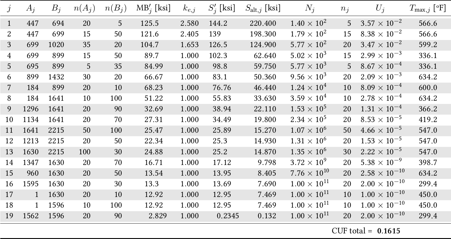{#fig:cuf-seamplex width=100%}

Tables of individual usage factors for the NRC/EPRI “EAF Sample Problem 2-Rev.\ 2 (10/21/2011).” One table is taken from a document issued by almost-a-billion-dollar-year-budget government agency from the most powerful country in the world and the other one is from a third-world engineering startup :::::

Why all these details? Not because I want to teach you how to perform fatigue evaluations just reading this section without resorting to ASME, fatigue books and even other colleagues. It is to show that even though these computation can be made “by hand” (i.e. using a calculator or, God forbids, a spreadsheet) when having to evaluate a few SCLs within several piping systems it is far (and I mean really far) better to automatise all these steps by writing a set of scripts. Not only will the time needed to process the information be reduced, but also the introduction of human errors will be minimised and repeatability of results will be assured---especially if working under a distributed version control system such as Git. This is true in general, so here is another tip: learn to write scripts to post-process your FEM results (you will need to use a script-friendly FEM program) and you will gain considerable margins regarding time and quality.

In water (NRC’s extension)

The fatigue curves and ASME’s (both\ III and VIII) methodology to analyse cyclic operations assume the parts under study are in contact with air, which is not the case of nuclear reactor pipes. Instead of building a brand new body of knowledge to replace ASME, the NRC decided to modify the former adding environmentally-assisted fatigue multipliers to the traditional usage factors, formally defined as

$$F\text{en} = \frac{N\text{air}}{N_\text{water}} \geq 1$$

This way, the environmentally-assisted usage factor for the $j$-th load pair is

$$\text{CUF}_\text{en,j} = Uj \cdot {F\text{en},j}$$ and the global cumulative usage factor in water is the sum of these partial contributions

$$\text{CUF}_\text{en} = U1 \cdot F{\text{en},1} + U2 \cdot F{\text{en},2} + \dots + Uj \cdot F{\text{en},j} + \dots$${#eq:cufen}

In EPRI’s words:

The general steps for performing an EAF analysis are as follows:

1. perform an ASME fatigue analysis using fatigue curves for an air environment
2. calculate $F_\text{en}$ factors for each transient pair in the fatigue analysis
3. apply the $F_\text{en}$ factors to the incremental usage calculated for each transient pair ($Uj$), to determine the $\text{CUF}\text{en}$, using\ [@eq:cufen]

Again, if $\text{CUF}\text{en} < 1$, then the system under study can withstand the assumed cyclic loads. Note that as\ $F{\text{en},j}$, we can have $\text{CUF} < 1$ and $\text{CUF}_\text{en} > 1$ at the same time.

\medskip

The NRC has performed a comprehensive set of theoretical and experimental tests to study and analyse the nature and dependence of the non-dimensional correction factors\ $F_\text{en}$. They found that, for a given material, they depend on:

a. the concentration\ $O(t)$ of dissolved oxygen in the water, b. the temperature\ $T(t)$ of the pipe, c. the strain rate\ $\dot{\epsilon}(t)$, and d. the content of sulphur\ $S(t)$ in the pipes (only for carbon or low-allow steels).

Apparently it makes no difference whether the environment is composed of either light or heavy water. There are somewhat different sets of non-dimensional analytical expressions that estimate the value of\ $F{\text{en}}(t)$ as a function of\ $O(t)$, $T(t)$, $\dot{\epsilon}(t)$ and $S(t)$, both in the few revisions of NUREG/CR-6909 and in EPRI’s report #1025823. Although they are not important now, the actual expressions should be defined and agreed with the plant owner and the regulator. The main result to take into account is that\ $F{\text{en}}(t)=1$ if\ $\dot{\epsilon}(t)\leq0$, i.e. there are no environmental effects during the time intervals where the material is being compressed.

Once we have the instantaneous factor\ $F{\text{en}}(t)$, we need to obtain an average value\ $F{\text{en},j}$ which should be applied to the\ $j$-th load pair. Again, there are a few different ways of lumping the time-dependent\ $F{\text{en}}(t)$ into a single $F{\text{en},j}$ for each interval. Both NRC and EPRI give simple equations that depend on a particular time discretisation of the stress histories that, in my view, are all ill-defined. My guess is that they underestimated they audience and feared readers would not understand the slightly-more complex mathematics needed to correctly define the problem. The result is that they introduced a lot of ambiguities (and even technical errors) just not to offend the maths illiterate. A decision I do not share, and a another reason to keep on learning and practising math.

When faced for the first time with the case study, I have come up with a weighting method that I claim is less ill-defined (it still is for border-line cases) and which the plant owner accepted as valid. [@Fig:cufen] shows the reference results of the problem (based on computing two correction factors and then taking the maximum) and the ones obtained with the proposed method (by computing a weighted integral between the valley and the peak). Note how in\ [@fig:cufen-nrc], pairs 694-447 and 699-447 have the same\ $F_\text{en}$ even though they are (marginally) different. The results from\ [@fig:cufen-seamplex] give two (marginally) different correction factors.

::::: {#fig:cufen} {#fig:cufen-nrc width=75%}

{#fig:cufen-seamplex width=75%}

Tables of individual environmental correction and usage factors for the NRC/EPRI “EAF Sample Problem 2-Rev.\ 2 (10/21/2011).” The reference method assigns the same\ $F_\text{en}$ to the first two rows whilst the proposed lumping scheme does show a difference :::::

Conclusions

Back in college, we all learned how to solve engineering problems. And once we graduated, we felt we could solve and fix the world (if you did not graduate yet, you will feel it shortly). But there is a real gap between the equations written in chalk on a blackboard (now probably in the form of beamer slide presentations) and actual real-life engineering problems. This chapter introduces a real case from the nuclear industry and starts by idealising the structure such that it has a known analytical solution that can be found in textbooks. Additional realism is added in stages allowing the engineer to develop an understanding of the more complex physics and a faith in the veracity of the finite-element results where theoretical solutions are not available. Even more, a brief insight into the world of evaluation of stress-life fatigue using such results further illustrates the complexities of real-life engineering analysis.

A list of the tips that arose throughout the text:

• use and exercise your imagination
• practise math
• start with simple cases first
• grasp the dependence of results with independent variables
• keep in mind there are other methods beside finite elements
• take into account that even within the finite element method, there is a wide variety of complexity in the problems that can be solved
• follow the “five whys rule” before compute anything, probably you do not need to
• use engineering judgment and make sure understand the “wronger than wrong” concept
• play with your favourite FEM solver (mine is CAEplex) solving simple cases, trying to predict the results and picturing the stress tensor and its eigenvectors in your imagination
• try to show that even though the principal stresses are not linear with respect to summation, they are linear with respect to multiplication (with pencil and paper)
• grab any stress distribution from any of your FEM projects, compute the iso-stress curves and the draw normal lines to them to get acquainted with SCLs
• first search online for “stress linearisation” (or “linearization” if you want) and then get a copy of ASME\ VIII Div\ 2 Annex 5-A
• keep in mind that FEM solutions lead only to nodal equilibrium but not pointwise equilibrium
• measure the time needed to generate grids of different sizes and kinds with your favourite mesher
• learn this by heart: the complexity of a FEM problem is given mainly by the number of nodes, not by the number of elements
• remember that welded materials with different thermal expansion coefficients may lead to fatigue under cyclic temperature changes
• if you have time, try to get out of your comfort zone and do more than what others expect from you (like parametric computations)
• clone the parametric tee repository, understand how the figures from\ [@sec:parametric] were built and expand them to cover “we might go on…” bullets
• try to find an explanation of the results obtained, just like we did when we explained the parametric curves from\ [@fig:tee-MB ] with two opposing effects which were equal in magnitude around $d_b=5$\ inches
• think thermal-mechanical plus earthquakes as “bake, break and shake” problems
• understand why the elastic problem of the case study is still linear after all
• keep in mind that finite-elements are a mean to get an engineering solution, not and end by themselves
• learn to write scripts to post-process FEM results (from a script-friendly FEM program)
• work under a distributed version control system such as Git, even when just editing input files or writing reports
• clone the environmental fatigue sample problem repository and obtain a nicely-formatted table with the results of the “EAF Sample Problem 2-Rev.\ 2 (10/21/2011)” from\ [@sec:in-air;@sec:in-water].
• do not write ambiguous reports by replacing appropriate mathematical formulae with words just not to offend the illiterate
• try to avoid proprietary programs and favour free and open source ones.

You can ask for help in our mailing list at wasora@seamplex.com. There is a community of engineers willing to help you in case you get in trouble with the repositories, the script or the input files.

About your favourite FEM program, ask yourself these two questions:

1. Does your favourite FEM program’s manual say what the program does?
2. Do you believe your favourite FEM program’s manual?
3. Do you trust your favourite FEM program?

And finally, make sure that at the end of the journey from college theory to an actual engineering problem your conscience, is clear knowing that there exists a report with your signature on it. That is why we went to college in the first place.

divert(-1)

Referenced works

Books

Articles

Reports

Blog posts

Websites

esyscmd(lynx -dump -listonly nafems4.html )

Wikipedia

esyscmd(lynx -dump -listonly nafems4.html ) divert(0)

---

1. The dean of the engineering school I attended used to say “It is not the same to read than to write manuals, and we should aim at writing them.”
2. A former boss once told me “I need the CFD” when I handed in some results. I replied that I did not do computational fluid-dynamics but computed the neutron flux kinetics within a nuclear reactor core. He joked “I know, what I need are the Colors For Directors, those pretty-coloured figures along with your actual results to convince the managers.”
3. https://www.seamplex.com/fino/doc/pipe-linearized/
4. https://bitbucket.org/seamplex/tee
5. https://bitbucket.org/seamplex/cufen