nafems4/nafems4.md

Background and introduction

First of all, please take this text as a written chat between you an me, i.e. an average engineer that have already taken the journey from college to performing actual engineering using finite element analysis and has something to say about it. Picture yourself in a coffee bar, talking and discussing concepts and ideas with me. Maybe needing to go to a blackboard (or notepad?). Even using a tablet to illustrate some three-dimensional results. But always as a chat between colleagues.

Please also note that I am not a mechanical engineer, although I shared many undergraduate courses with some of them. I am a nuclear engineer with a strong background on mathematics and computer programming. I went to college between 2002 and 2008. Probably a lot of things have changed since then---at least that is what these “millenials” guys and girls seem to be boasting about---but chances are we all studied solid mechanics and heat transfer with a teacher using a piece of chalk on a blackboard and students writing down notes with pencils on paper sheets. And there is really not much that one can do with pencil and paper regarding mechanical analysis. Any actual case worth the time of an engineer need to be more complex than an ideal canonical case with analytical solution.

We will be swinging back and forth between a case study about fatigue analysis in piping systems of a nuclear power plant and more generic and even romantic topics related to finite elements and computational mechanics. These latter regressions will not remain just as abstract theoretical ideas. Not only will they be directly applicable to the development of the main case, but they will also apply to a great deal of other engineering problems tackled with the finite element method.

Finite elements are like magic to me. I mean, I can follow the whole derivation of the equations, from the strong, weak and variational formulations of the equilibrium equations for the mechanical problem (or the energy conservation for heat transfer) down to the algebraic multigrid preconditioner for the inversion of the stiffness matrix passing through Sobolev spaces and the grid generation. Then I can sit down and program all these steps into a computer, including the shape functions and its derivatives, the assembly of the discretised stiffness matrix assembly, the numerical solution of the system of equations and the computation of the gradient of the solution. Yet, the fact that all these a-priori unconnected steps once gets a pretty picture that resembles reality is still astonishing to me.

Again, take all this information as coming from a fellow that has already taken such a journey from college’s pencil and paper to real engineering cases involving complex numerical calculations. And developing, in the meantime, both an actual working finite-element back-end and front-end from scratch.

Tips and tricks

There are some useful tricks that come handy when trying to solve a mechanical problem. Throughout this text, I will try to tell you some of them.

One of the most important ones is using your imagination. You will need a lot of imagination to “see“ what it is actually going on when analysing an engineering problem. This skill comes from my background in nuclear engineering where I had not choice but to imagine a positron-electron annihilation or an Spontaneous fission. But in mechanical engineering, it is likewise important to be able to imagine how the loads “press” one element with the other, how the material reacts depending on its properties, how the nodal displacements generate stresses (both normal and shear), how results converge, etc. And what these results actually mean besides the pretty-coloured figures.¹ This journey will definitely need your imagination. We will see equations, numbers, plots, schematics, 3D geometries, interactive 3D views, etc. Still, when the theory says “thermal expansion produces linear stresses” you have to picture in your head three little arrows pulling away from the same point in three directions, or whatever mental picture you have about what you understand are thermally-induced stresses. What comes to your mind when someone says that out of the nine elements of the stress tensors there are only six that are independent? Whatever it is, try to practice that kind of graphical thoughts with every concept.

Another heads up is that we will dig into some math. Probably it would be be simple and you would deal with it very easily. But probably you do not like equations. No problem! Just ignore them for now. Read the text skipping them, it should work. It is fine to ignore math (for now). But, eventually, a time will come in which it cannot (or should not) be avoided. Here comes another experience tip: do not fear mathematics. Even more, keep exercising. You have used differences of squares in high school. You know (or at least knew) how to integrate by parts. Remember what Laplace transforms are used for? Once in a while, perform a division of polynomials using Ruffini’s rule. Or compute the second derivative of the quotient of two functions. Whatever. It should be like doing crosswords on the newspaper. Grab those old physics college books and read the exercises at the end of each chapter. It will pay off later on.

Case study: nuclear reactors, pressurised pipes and fatigue

Piping systems in sensitive industries like nuclear or oil & gas should be designed and analysed following the recommendations of an appropriate set of codes and norms, such as the ASME\ Boiler and Pressure Vessel Code. This code of practice (book) was born during the late\ XIX century, before finite-element methods for solving partial differential equations were even developed. And much longer before they were available for the general engineering community. Therefore, much of the code assumes design and verification is not necessarily performed numerically but with paper and pencil (yes, like in college). However, it still provides genuine guidance in order to ensure pressurised systems behave safely and properly without needing to resort to computational tools. Combining finite-element analysis with the ASME code gives the cognisant engineer a unique combination of tools to tackle the problem of designing and/or verifying pressurised piping systems.

In the years following Enrico Fermi’s demonstration that a self-sustainable fission reaction chain was possible (actually, in fact, after WWII was over), people started to build plants in order to transform the energy stored within the atoms nuclei into usable electrical power. They quickly reached the conclusion that high-pressure heat exchangers and turbines were needed. So they started to follow the ASME\ Boiler and Pressure Vessel Code. They also realised that some requirements did not fit the needs of the nuclear industry. But instead of writing a new code from scratch, they added a new chapter to the existing body of knowledge: the celebrated ASME Section\ III.

After further years passed by, engineers (probably the same people that forked section\ III) noticed that fatigue in nuclear power plants was not exactly the same as in other piping systems. There were some environmental factors directly associated to the power plant that was not taken into account by the regular ASME code. Again, instead of writing a new code from scratch, people decided to add correction factors to the previously amended body of knowledge. This is how knowledge evolves, and it is this kind of complexities that engineers are faced with during their professional lives. We have to face it, it would be a very hard work to re-write everything from scratch every time something changes.

{#fig:real-life}

Actually, this article does not focus on a single case study but on some general ideas regarding analysis of fatigue in piping systems in nuclear power plants. There is no single case study but a compendium of ideas obtained by studying many different systems which are directly related to the safety of a real nuclear reactor.

Nuclear reactors

In each of the countries that have at least one nuclear power plant there exists a national regulatory body who is responsible for allowing the owner to operate the reactor. These operating licenses are time-limited, with a range that can vary from 25 to 60 years, depending on the design and technology of the reactor. Once expired, the owner might be entitled to an extension, which the regulatory authority can accept provided it can be shown that a certain (and very detailed) set of safety criteria are met. One particular example of requirements is that of fatigue in pipes, especially those that belong to systems that are directly related to the reactor safety.

Pressurised pipes

How come that pipes are subject to fatigue? Well, on the one hand and without getting into many technical details, the most common nuclear reactor design uses liquid water as coolant and moderator. On the other hand, nuclear power plants cannot by-pass the thermodynamics of the Carnot cycle, and in order to maximise the efficiency of the conversion between the energy stored in the uranium nuclei into electricity they need to reach temperatures as high as possible. So, if we want to have liquid water in the core as hot as possible, we need to increase the pressure. The limiting temperature and pressure are given by the critical point of water, which is around 374ºC and 22\ MPa. It is therefore expected to have temperature and pressures near those values in many systems of the plant, especially in the primary circuit those that directly interact with it, such as pressure and inventory control system, decay power removal system, feedwater supply system, emergency core-cooling system, etc.

Nuclear power plants are not always working at 100% power. They need to be maintained and refueled, they may undergo operational transients, they might operates at a lower power due to load following conditions, etc. These transient cases involved changes both in temperatures and in pressures that the pipes are subject to, which in turn give rise to changes in the stresses within the pipes. As the transients are postulated to occur conservatively cyclically during a number of times during the life-time of the plant (plus its extension period), mechanical fatigue in these piping systems arise especially at the interfaces between materials with different thermal expansion coefficients.

An important part of the analysis that almost always applies to nuclear power plants but usually also to other installations is the consideration of a possible seismic event. Given a postulated design earthquake, the civil structures that hold the pipes have a response spectra for each floor level. One has to combine these spectra with the natural oscillation modes and frequencies of the piping system using one of several available methodologies such as the “Square Root of Sum of Squares” or SRSS method. This way, an static-equivalent distributed internal load can be computed and then applied as extra loads conservatively (see [@sec:kinds]) at the moment of highest mechanical demand.

Fatigue

Mechanical systems can fail due to a wide variety of reasons. The effect known as fatigue can create, migrate and grow microscopic cracks at the atomic level, called dislocations. Once these cracks reach a critical size, then the material fails catastrophically even under stresses lower than tensile strength limits. There are not complete mechanistic models from first principles which can be used in general situations, and those that exist are very complex and hard to use. Instead, using an experimental approach very much like the Hooke Law experiment, the stress amplitude of a periodic cycle can be related to the number of cycles where failure by fatigue is expected to occur. For each material, this dependence can be computed using normalised tests and a family of “fatigue curves” (also called $S$-$N$ curves) for different temperatures can be obtained.

It should be stressed that the fatigue curves are obtained in a particular load case, namely purely-periodic one-dimensional, which is not directly generalised to other three-dimensional cases. The application of the curve data implies a set of simplifications and assumptions that are translated into different possible “rules” for composing real-life cycles. There also exist two safety factors which increase the stress amplitude and reduce the number of cycles respectively. All these intermediate steps render the analysis of fatigue into a conservative computation scheme. Therefore, when a fatigue analysis performed using the fatigue curve method arrives at the conclusion that “fatigue is expected to occur after ten thousand cycles” what it actually means is “we are sure fatigue will not occur before ten thousand cycles, yet it may not occur before one hundred thousand or even more.”

Solid mechanics, or what we are taught at college

So, let us start our journey. Our starting place: undergraduate solid mechanics courses. Our goal: to obtain the internal state of a solid subject to a set of movement restrictions and loads (i.e. to solve the solid mechanics problem). Our first step: Newton’s laws of motion. For each of them, all we need to recall here is that

1. a solid is in equilibrium if it is not moving in at least one inertial coordinate system,
2. in order for a solid not to move, the sum of all the forces ought to be equal to zero, and
3. for every external load there exists an internal reaction with the same magnitude but opposite direction.

We have to accept that there is certain intellectual beauty when complex stuff can be expressed in simple term. Yet, from now on, everything can be complicated at will. We can take the mathematical path like D’Alembert and his virtual displacements ideas (in his mechanical treatise, D’Alembert brags that he does not need to use a single figure throughout the book). Or we can go graphical following Cullman. Or whatever other logic reasoning to end up with a set of actual equations which we need to solve in order to obtain engineering results.

The stress tensor

In any case, what we should understand (and imagine) is that external forces lead to internal stresses. And in any three-dimensional body subject to such external loads, the best way to represent internal stresses is through a $3 \times 3$ stress tensor. This is the first point in which we should not fear math. Trust me, it will pay back later on.

Does the term tensor scare you? It should not. A tensor is just a slightly more complex vector, and I assume you are not afraid of vectors. If you recall, a vector somehow generalises the idea of a scalar in the following sense: a given vector $\vec{v}$ can be projected into any direction $\vec{n}$ to obtain a scalar $p$. We call this scalar $p$ the “projection” of the vector $\vec{v}$ in the direction $\vec{n}$. Well, a tensor can be also projected into any direction $\vec{n}$. The difference is that instead of a scalar, a vector is now obtained.

Let me introduce then the three-dimensional stress tensor:

$$ \begin{bmatrix} \sigmax & \tau{xy} & \tau{xz} \ \tau{yx} & \sigma{y} & \tau{yz} \ \tau{zx} & \tau{zy} & \sigma_{z} \ \end{bmatrix} $$

It looks (and works) like a regular $3 \times 3$ matrix. Some brief comments about it:

• The $\sigma$s are normal stresses, i.e. they try to stretch or tighten the material.
• The $\tau$s are shear stresses, i.e. they try to twist the material.
• It is symmetric (so there are only six independent elements) because
  • $\tau{xy} = \tau{yx}$,
  • $\tau{yz} = \tau{zy}$, and
  • $\tau{zx} = \tau{xz}$.
• The elements of the tensor depends on the orientation of the coordinate system.
• There exists a particular coordinate system in which the stress tensor is diagonal, i.e. all the shear stresses are zero. In this case, the three diagonal elements are called the principal stresses.

What does this all have to do with mechanical engineering? Well, once we know what the stress tensor is for every point of a solid, in order to obtain the internal forces per unit area acting in a plane passing through that point and with a normal given by the direction $\vec{n}$, all we have to do is “project” the stress tensor through $\vec{n}$. In plain simple words:

• If you can compute the stress tensor at each point of our geometry, then… Congratulations! You have solved the solid mechanics problem.

An infinitely-long pressurised pipe

Let us proceed to a our second step, and consider an infinite pipe subject to uniform internal pressure. Actually, we are going to solve the mechanical problem on an infinite hollow cylinder, which looks like pipe. This case is usually tackled in college courses, and chances are you already solved it. Actually, the first (and simpler) problem is the “thin cylinder problem.” Then, the “thick cylinder problem” is introduced, which is slightly more complex. Nevertheless, it has an analytical solution which is derived here. For the present case, Let us consider an infinite pipe (i.e. a hollow cylinder) of internal radius $a$ and external radius $b$ with uniform mechanical properties---Young modulus $E$ and Poisson’s ratio $\nu$---subject to an internal uniform pressure $p$.

Displacements

Remember that when any solid body is subject to external forces, it has to reach in such a way to satisfy the equilibrium conditions. The way solids do this is by deforming a little bit in such a way that the whole body acts as a compressed (or elongated) spring balancing the load. So it is worth to ask how a pressurized pipe deforms to counteract the internal pressure\ $p$.

• There are no longitudinal displacements\ $u_l$ because the pipe is infinite in the axial direction.
• There are no azimuthal displacements\ $u_\theta$ because the pipe is fully symmetric around the axis.
• There are only radial displacements\ $u_r$ and they depend only on the radial coordinate\ $r$ and not on the axial position\ $z$ or on the azimuthal angle\ $\theta$. This displacements are

$$ u_r® = p \cdot \frac{1+\nu}{E} \cdot \frac{a^2}{b^2-a^2} \cdot \left[ 1-2\nu + \frac{b^2}{r^2} \right]\cdot r $$

What does this mean? Well, that overall the whole pipe expands a little bit radially with the inner face being displaced more than the external surface (use your imagination!). How much?

1. Linearly with the pressure, i.e. twice the pressure, twice the displacement, and
2. Inversely proportional to the Young Modulus\ $E$ divided by $1+\nu$, i.e. the more resistant the material, the less radial displacements.

That is how an infinite pipe withstands internal pressure.

Stresses

As the solid is deformed, that is to say that different parts are relatively displaced one from another, strains and stresses appear. When seen from a cylindrical coordinate system, the stress tensor (recall [@sec:tensor]) has these features.

• There are no shear stresses as there is no bending due to the fact that the pipe is infinite (so it cannot bend in the axial direction) and azimuthally symmetric (there is no particular direction so circles must remain circles).

• The normal stresses depend only on the radial coordinate\ $r$ and are

  • the radial stress\ $\sigma_r$,

  $$ \sigma_r® = \frac{p \cdot a^2}{b^2-a^2} \cdot \left( 1 - \frac{b^2}{r^2}\right) $$ {#eq:sigmar}

  • the azimuthal (or hoop) stress\ $\sigma_\theta$, and

  $$ \sigma_\theta® =\frac{p \cdot a^2}{b^2-a^2} \cdot \left( 1 + \frac{b^2}{r^2}\right) $$ {#eq:sigmatheta}

  • the longitudinal (or axial) stress\ $\sigma_l$.

  $$ \sigma_l® = 2\nu \cdot \frac{p \cdot a^2}{b^2-a^2} $${#eq:sigmal}

We can note that

1. The stresses do not depend on the mechanical properties\ $E$ and\ $\nu$ of the material (the displacements do).
2. All the stresses are linear with the pressure\ $p$, i.e. twice the pressure, twice the stress.
3. The axial stress is uniform and does not depend on the radial coordinate\ $r$.
4. As the stress tensor is diagonal, these three stresses happen to also be the principal stresses.

That is all what we can say about an infinite pipe with uniform material properties subject to an uniform internal pressure\ $p$. If

• the pipe was not infinite (say any real pipe that has to start and end somewhere), or
• the cross-section of the pipe is not constant along the axis (say there is a reduction), or
• there was more than one pipe (say there is a tee), or
• the material properties are not uniform (say the pipe does not have an uniform temperature but a distribution), or
• the pressure was not uniform (say because there is liquid inside and its weight cannot be neglected),

\noindent then we would no longer be able to fully solve the problem with paper and pencil and draw all the conclusions above. However, at least we have a start because we know that if the pipe is finite but long enough or the temperature is not uniform but almost, we still can use the analytical equations as approximations. After all, Enrico Fermi managed to reach criticality in the Chicago Pile-1 with paper and pencil. But what happens if the pipe is short, there are branches and temperature changes like during a transient in a nuclear reactor? Well, that is why we have finite elements. And this is were what we learned at college ends.

Finite elements, or solving an actual engineering problem

Besides infinite pipes (both thin and thick), spheres and a couple of other geometries, there are not other cases for which we can obtain analytical expressions for the elements of the stress tensor. To get results for a solid with real engineering interest, we need to use numerical methods to solve the equilibrium equations. It is not that the equations are hard per se. It is that the mechanical parts we engineers like to design (which are of course better than cylinders and spheres) are so intricate that render simple equations into monsters which are unsolvable with pencil and paper. Hence, finite elements enter into the scene.

The name of the game

But before turning our attention into finite elements (and leaving college, at least undergraduate) it is worth some time to think about other alternatives. Are we sure we are tackling your problems in the best possible way? I mean, not just engineering problems. Do we take a break, step back for a while and see the whole picture looking at all the alternatives so we can choose the best cost-effective one?

There are literally dozens of ways to numerically solve the equilibrium equations, but for the sake of brevity let us take a look at the three most famous ones. Coincidentally, they all contain the word “finite” in their names. We will not dig into them, but it is nice to know they exist. We might use

1. Finite differences
2. Finite volumes
3. Finite elements

Each of these methods (also called schemes) have of course their own features, pros and cons. They all exploit the fact that the equations are easy to solve in simple geometries (say a cube). Then the actual geometry is divided into a yuxtaposition of these cubes, the equations are solved in each one and then a global solution is obtained by sewing the little simple solutions one to another. The process of dividing the original domain into simple geometries is called discretization, and the resulting collection of these simple geometries is called a mesh or grid. They are composed of volumes, called cells (or elements) and vertices called nodes. Now, grids can be either

a. structured, or b. unstructured

Figure [-@fig:grids] illustrates how the same domain can be discretized using these two kind of grids. In the first case, we could identify any single cell by using just two indexes. We could even tell which nodes define each cell just from these indexes. In the second case, we need an explicit list first to know how many cells there are. Even more, there is no way to link the nodes with the cells (back and forth) other than having a list of nodes and cells. Again, there are pros and cons for each of the grid types such as simplicity, flexibility, etc. In general, unstructured grids and better represent a certain geometry with the same number of cells. Structured grids suffer the so-called “staircase effect” that makes the unusable for discretizing mechanical parts.

::::: {#fig:grids} {#fig:continuous width=30%} {#fig:structured width=30%} {#fig:unstructured width=30%}

Discretization of a spatial domain :::::

The first of the three methods is based on approximating derivative (i.e. differentials) by incremental quotients (i.e. differences). The second one heavily relies on geometrical ideas rather than on pure mathematical grounds. Finally, our beloved finite elements are the most “mathematical” ones. Actually, a complete derivation of the finite element method can be written in a textbook without requiring a single figure, just like D’Alembert did more than two centuries ago. In any case, it is important to note that finite differences and elements compute results at the nodes of a mesh, whilst finite volumes compute results at the cells of a mesh. Finally, any method may be used in structured grids but only finite elements and volumes are especially suited for working with unstructured grids.

There are technical reasons that justify why the finite element method is the king of mechanical analysis. But that does not mean that other methods may be employed. For instance, fluid mechanics are better solved using finite volumes. And further other combinations may be found in the literature.

Before proceeding, I would like to make two comments about common nomenclature. The first one is that if we exchanged the words “volumes” and “elements” in all the written books and articles, nobody would note the difference. There is nothing particular in both theories that can justify why finite volumes use volumes and finite elements use elements. Actually volumes and elements are the same geometric constructions. The names were randomly assigned.

The second one is more philosophical and refers to the word “simulation” which is often used to refer to solving a problem using a numerical scheme such as the finite element method. I am against at using this word to refer to this endeavour. The term simulation has a connotation of both “pretending” and “faking” something, that is definitely not what we are doing when solving an engineering problem with finite elements. Sure there are some cases in which we simulate, such as using the Monte Carlo method (originally used by Fermi as an attempt to understand how neutrons behave in the core of nuclear reactors). But when solving deterministic mechanical engineering problems I would rather say “modelling” than “simulation.”

Kinds of finite elements

This section is not (just) about different kinds of elements like tetrahedra, hexahedra, pyramids and so on. It is about the different kinds of analysis there are. Indeed, there are a whole plethora of particular types of calculations we can perform, all of which can be called “finite element analysis.” For instance, for the mechanical problem, we can have different kinds of

• temporal dependence
  • steady-state
  • quasi-static
  • transient
• main elements
  • 1D beam elements
  • 2D shell elements
  • 3D bulk elements
• mathematical models
  
  • pure linear
  • material non-linear
  • geometrical non-linear
• particular studies
  • buckling
  • modal
• element features
  • full elements
  • sub-integrated elements
  • incomplete elements

And then there exist different pre-processors, meshers, solvers, pre-conditioners, post-processing steps, etc. A similar list can be made for the heat conduction problem, electromagnetism, the Schröedinger equation, neutron transport, etc. But there is also another level of “kind of problem,” which is related to how much accuracy and precision we are to willing sacrifice in order to have a (probably very much) simpler problem to solve. Again, there are different combinations here but a certain problem can be solved using any of the following three approaches, listed in increasing amount of difficulty and complexity:

i. conservative ii. best-estimate iii. probabilistic

The first one is the easiest because we are allowed to choose parameters and to make engineering decisions that may simplify the computation as long as they give results towards the worse-case scenario. More often than not, an conservative estimation is enough in order to consider a problem solved. Note that this is actually how fatigue results are obtained using fatigue curves, as discussed in\ [@sec:fatigue]. A word of care should be taken when considering what the “worst-case scenario” is. For instance, if we are analysing the temperature distribution in a mechanical part subject to convection boundary conditions, we might take either a very large or a very low convection coefficient as the conservative case. If we needed to design fins to dissipate heat then a low coefficient would be the choice conservative. But if the mechanical properties deteriorated with high temperatures then the conservative way to go would be to set a high convection coefficient. A common practice is to have a fictitious set of parameters, each of them being conservative leading individually to the worst-case scenario even if the overall combination is not physically feasible.

As neat and tempting as conservative computations may be, sometimes the assumptions may be too biased toward the worst-case scenario and there might be no way of justifying certain designs with conservative computations. It is then time to sharpen our pencils and perform a best-estimate computation. This time, we should stick to the most-probable values of the parameters and even use more complex models that can better represent the physical phenomena that are going on in our problem. Sometimes best-estimate computations are just slightly more complex than conservative models. But more often than not, best-estimates get far more complicated. And these complications come not just in the finite-element model of the elastic problem but in the dependence of properties with space, time and/or temperature, in non-trivial relationships between macro and microscopic parameters, in more complicated algorithms for post-processing data, etc.

Example?

Finally, when then uncertainties associated to the parameters, methods and models used in a best-estimate calculation render the results too inaccurate for a certain regulatory body to approve a design, it might be needed to do a full set of parametric runs taking into account the probabilistic distribution of each of the input parameters. This kind of computation involve

1. a thorough analysis of the probability densities of the parameters (and even the methods) of a problem,
2. performing a large number of runs for different combination of parameters, and
3. combining all the results into to obtain a best-estimate value plus uncertainty.

This kind of computation is usually required by the nuclear regulatory authorities when power plant designers need to address the safety of the reactors. What is the heat capacity of uranium above 1000ºC? What is the heat transfer coefficient when approaching the critical heat flux before the Leidenfrost effect occurs? A certain statistical analysis has to be done prior to actually parametrically swifting the input parameters so as to obtain a distribution of possible outcomes.

Five whys

So we know we need a numerical scheme to solve our mechanical problem because anything slightly more complex than an infinite pipe does not have analytical solution. We need an unstructured grid because we would not use Legos to discretise pipes. We selected the finite elements method over the finite volumes method, because FEM is the king. Can we pause again and ask ourselves why is it that we want to do finite-element analysis?

There exists a very useful problem-solving technique coined by Taiichi Ohno, the father of the Toyota production system, known as the Five-whys rule. It is based on the fact people make decisions following a certain reasoning logic that most of the time is subjective and biased and not purely rational and neutral. By recursively asking (at least five times) the cause of a certain issue, it might possible to understand what the real nature of the problem (or issue being investigated) is. And it might even be possible to to take counter-measures in order to fix what seems wrong.

Here is an original example:

1. Why did the robot stop?
   The circuit has overloaded, causing a fuse to blow.

2. Why is the circuit overloaded?
   There was insufficient lubrication on the bearings, so they locked up.

3. Why was there insufficient lubrication on the bearings?
   The oil pump on the robot is not circulating sufficient oil.

4. Why is the pump not circulating sufficient oil?
   The pump intake is clogged with metal shavings.

5. Why is the intake clogged with metal shavings?
   Because there is no filter on the pump.

You get the point. We usually assume we have to do what we usually do (i.e. perform finite element analysis). But do we? Do we add a filter or just replace the fuse?

Getting back to the case study: do we need to do FEM analysis? Well, it does not look like we can obtain the stresses the transient cases with just pencil and paper. But how much complexity should we add? We might do as little as axysimmetric linear steady-state conservative studies or as much as full three-dimensional non-linear transient best-estimate plus uncertainties computations. And here is where good engineers should appear: in putting their engineering judgment (call it experience or hunches) into defining what to solve. And it is not (just) because the first option is faster to solve than the latter. Involving many complex methods need more engineering time

1. to prepare the input data and set up the algorithms, and
2. to analyse the output data and write engineering reports.

In the first years of the history of computer, when programs where written in decks and output results were printed in continuous paper sheets, it made sense for computer programs to calculate and write as much data as possible even if it was not needed. One would never know if it would not be needed in the future, and CPU time was so expensive that re-running engineering computations because a results was not included in the output was forbidden. But that is not remotely true in the XXI century anymore. Computing time is far cheaper than engineering time (result known as the UNIX Rule of Economy) that it should be neglected with respect to the time spent by a cognizant engineer searching and sorting thousands of hard-to-read floating-point numbers.

divert(-1)

---

Computers, those little magic boxes

When we think about finite elements, we automatically think about computers. Of

https://www.springfieldspringfield.co.uk/view_episode_scripts.php?tv-show=the-simpsons&episode=s05e03

ENIAC

A brief review of history

FEM, Computers

graphics cards

Hardware

Software

FOSS

Avoid black boxes

Reflections on trusting trust

UNIX, scriptability, make programs to make programs (here a program is a calculation)

front and back

avoid monolithic

---

divert(0)

Piping in nuclear rectors

So we need to address the issue of fatigue in nuclear reactor pipes that

1. are not infinite and have cross-section changes, branches, valves, etc.
2. are made of different materials,
3. are fixed at different locations to the wall through piping supports,
4. are subject to a. pressure transients, b. heat transients, and c. seismic loads.

As I wanted to illustrate in [@sec:five], it is very important to decide what kind of problem (actually problems) we should be dealing with. As a nuclear engineer, I learned (theoretically in college but practically after college) that there are some models that let you see some effects and some that let you see other effects.² And even if, in principle, it is true that more complex models should let you see more stuff, they definitely might show you nothing at all if the model is so big and complex that it does not fit into a computer (say because it needs hundreds of gigabytes of RAM to run) or because it takes more time to compute than you may have before the final report is expected.

First of all, we should note that we need to solve

i. the heat transfer equation to get the temperature distribution within the pipes, ii. a frequency analysis of the piping system to get the natural oscillation modes and use them to obtain the pseudo-accelerations created by the design earthquake, and finally iii. the elastic problem to obtain the stress tensor needed to compute the alternating stress to enter into the fatigue curve.

So for each time of the operational transient, the pipes are subject to

a. an uniform internal pressure\ $p_i(t)$ that depends on time, b. a uniform internal temperature $T_i(t)$ that gives rise to a non-trivial time-dependent temperature distribution\ $T(\vec{x},t)$ in the bulk of the pipes, and c. internal distributed forces\ $\vec{f}=\rho \cdot \vec{a}$ at those times where the design earthquake is assumed to act.

Let us invoke our imagination once again. Assume in one part of the transients the temperature of the water inside the pipes falls from say 300ºC down to 100ºC in a couple of minutes, stays at 100ºC for another couple of minutes and then gets back to 100ºC. The temperature within the bulk of the pipes change as times evolves. The internal wall of the pipes follow the transient temperature (it might be exactly equal or close to it through the Newton’s law of cooling). If the pipe was in a state of uniform temperature, the ramp in the internal wall will start cooling the bulk of the pipe creating a transient thermal gradient. Due to thermal inertia effects, the temperature can have a non-trivial dependence when the ramps start or end (think about it!). So we need to compute a real transient heat transfer problem with convective boundary conditions because any other usual tricks like computing a sequence of steady-state computations for different times would not be able to recover these non-trivial distributions.

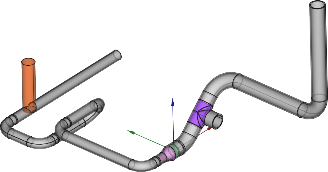
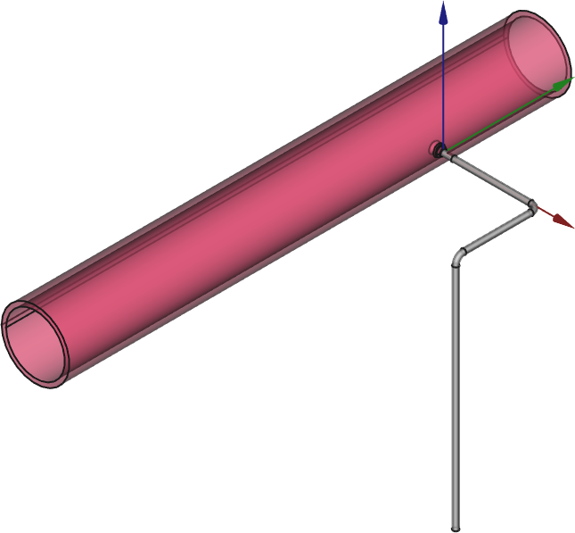
Remember the main issue of the fatigue analysis in these systems is to analyse what happens around the location of changes of piping classes where different materials (i.e. different expansion coefficients) are present, potentially causing high stresses due to differential thermal expansion (or contraction) under transient conditions. Therefore, even though we are dealing with pipes we cannot use beam or circular shell elements, because we need to take into account the three-dimensional effects of the temperature distribution along the pipe thickness. And even if it we could, there are some tees that connect pipes with different nominal diameters that have a non-trivial geometry, such as the weldolet-type junction shown in\ [@fig:weldolet-cad;@fig:weldolet-mesh]. In this case, there are a number of SCLs (Stress Classification Lines) that go through the pipe’s thickness at both sides of the material interface as illustrated in\ [@fig:weldolet-scls]. It is in these locations that fatigue is to be evaluated.

dnl 33410 07-3-4D-29

::::: {#fig:weldolet-cad} {#fig:weldolet-cad1}

{#fig:weldolet-cad2}

CAD model of a piping system with a ¾-inch weldolet-type fork (stainless steel) from a main 12-inch pipe (carbon steel). :::::

::::: {#fig:weldolet-mesh} {#fig:weldolet-mesh1}

{#fig:weldolet-mesh2}

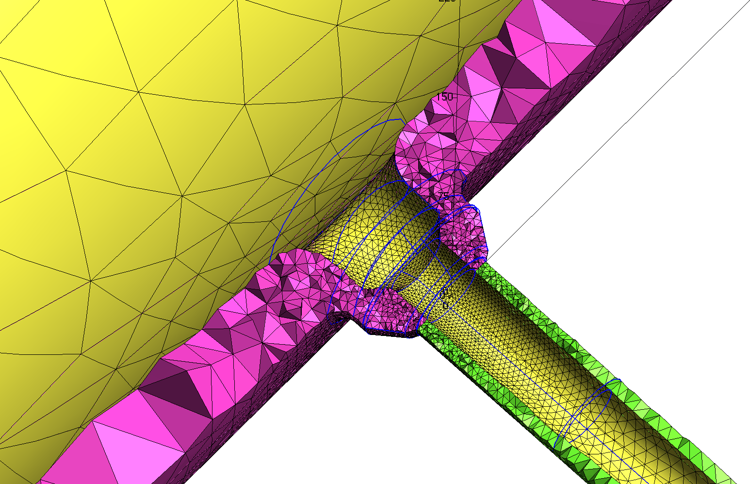
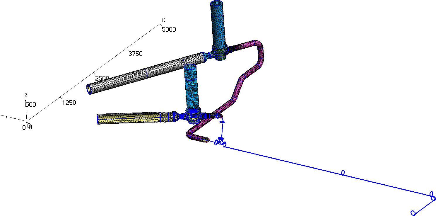
Three-dimensional unstructured tetrahedra-based grid for the system shown in\ [@fig:weldolet-cad] :::::

{#fig:weldolet-scls}

On the one hand, a reasonable number of nodes (remember it is the number of nodes that defines the problem size, not the number of elements) in order to get a decent grid is around 200k for each system. On the other hand, solving a couple of dozens of transient heat transfer problems (which we cannot avoid due to the large thermal inertia of the pipes) during a couple of thousands of seconds over a couple hundred of thousands of nodes might take more time and storage space to hold the results than we might expect.

There is a wonderful essay by Isaac Asimov called “The Relativity of Wrong” where he introduces the idea that even if something cannot be computed exactly, there are different levels of error. For instance, believing that the Earth is a sphere is less wrong than believing that the Earth is flat, but wrong nonetheless, since it really deviates from a perfect sphere and resembles more an oblate spheroid.

We can then merge this idea by Asimovve with an adapted version of the Saint-Venant’s principle and note that the detailed transient temperature distribution is important only around the location of the SCLs. We can then make an engineering approximation and

1. compute the transient thermal problem using a reduced mesh around the SCLs, and
2. assume the part of the full system which is not contained in the reduced mesh is at an uniform (though not constant) temperature equal to the average of the inner and outer temperatures at each side of the reduced mesh.

dnl 33300 02-D-3-4

::::: {#fig:valve} {#fig:valve-cad1}

{#fig:valve-mesh1}

{#fig:valve-scls1}

An example case where the SCLs are located around the junction with the stainless-steel valves and the carbon steel pipe. :::::

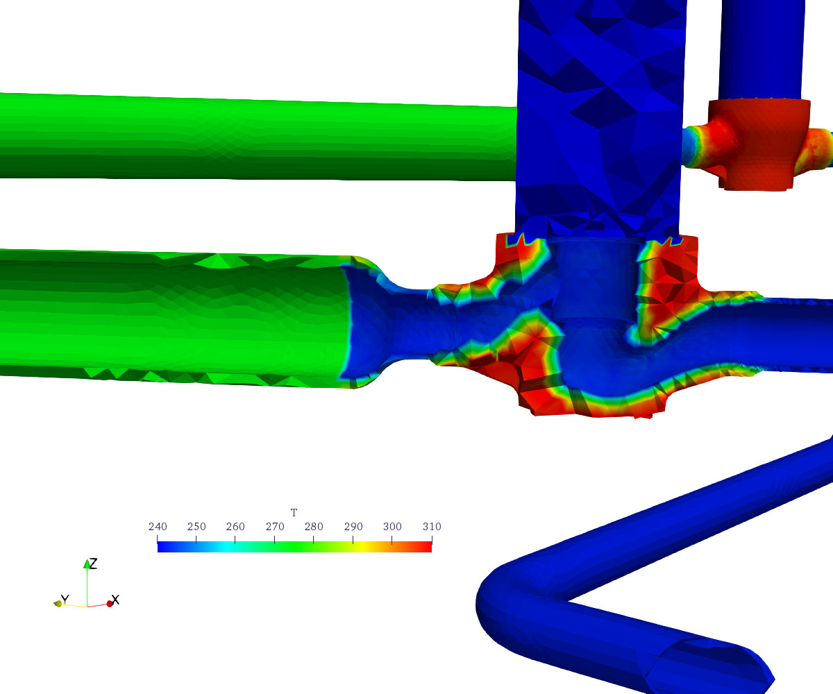
As an example, let us consider the system depicted in\ [@fig:valve-cad1;fig:valve-scls1] where there is a stainless-carbon steel interface at the discharge of the valves. Instead of solving the transient heat-conduction problem with the internal temperature of the pipes equal to the temperature of the water in the reference transient condition of the power plant and an external condition of natural convection to the ambient temperature in the whole mesh of\ [@fig:valve-mesh1], a reduced model consisting of half of one of the two valves and a small length of the pipes at both the valve inlet and outlet is used. Once the temperature distribution\ $\hat{T}(\vec{x},t)$ for each time is obtained in the reduced mesh ([@fig:valve-temp], which has the origin at the center of the valve), the actual temperature distribution\ $T(\vec{x},t)$ is computed by an algebraic genearalisation of $\hat{T}(\vec{x},t)$ in the full coordinate system (where the origin is shown in\ [@fig:valve-cad1]). As stated above, those locations which are not covered by the reduced model are generalised with a time-dependent uniform temperature which is the average of the inner and outer temperatures at the inlet and outlet of the reduced mesh. The result is illustrated in figure\ [@fig:valve-gen].

::::: {#fig:valve-temp-gen} {#fig:valve-temp}

{#fig:valve-gen}

Computation of the thermal problem in a reduced mesh and generalisation of the result to the full original 3D mesh of figure\ [@fig:valve-mesh1]. :::::

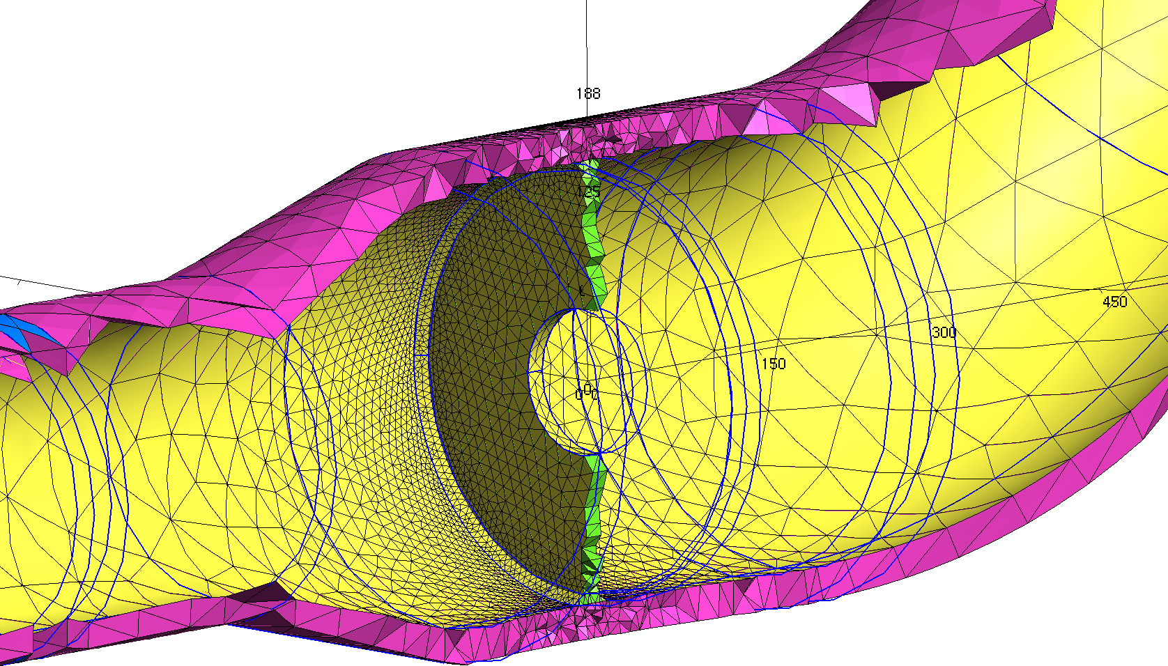
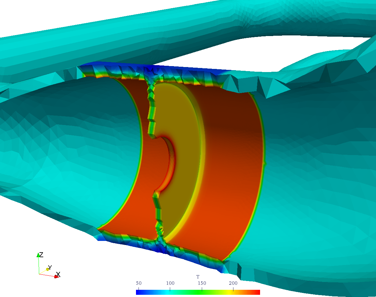
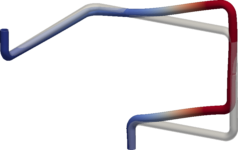
Please note that there is no need to have a one-to-one correspondence between the elements from the reduced mesh with the elements from the original one. Actually, the reduced mesh contains first-order elements whilst the former has quadratic tetrahedra. Also the grid density is different. Nevertheless, the finite-element solver Fino used both to solve the heat and the mechanical problems, allows to read functions of space and time defined over one mesh and continuously evaluate and use them into another one even if the two grids have different elements, orders or even dimensions. In effect, in the system from figure [@fig:real-life] the material interface is between a orifice plate made in stainless steel that is welded to a carbon-steel pipe ([@fig:real-mesh2]). The thermal problem can be modeled using a two-dimensional axisymmetric grid [@fig:real-temp] and then generalized to the full three-dimensional mesh using the algebraic manipulation capabilities provided by Fino (actually by wasora) as shown in\ [@fig:real-gen].

dnl 33410 10-12D-24

::::: {#fig:real} {#fig:real-mesh2}

{#fig:real-temp}

{#fig:real-gen}

The material interface in the system from [@fig:real-life] is configured by an orifice plate made of stainless steel welded to a carbon-steel pipe. :::::

Seismic loads

Before considering the actual mechanical problem that will give us the stress tensor at the SCLs and besides needing to solve the transient thermal problem to get the temperature distributions, we need to address the loads that arise due to a postulated earthquake during a certain part of the operational transients. The full computation of a mechanical transient problem using the earthquake time-dependent displacements is off the table for two reasons. First, because the computation would take more time than we might have to deliver the report. And secondly and more importantly, because civil engineers do not compute earthquakes in the time domain but in the frequency domain. Time to revisit our Laplace transform exercises from undergraduate math courses.

Earthquake spectra

In case you are wondering, the answer is yes: all nuclear power plants are designed to withstand earthquakes. Of course, not all plants need the same level of reinforcements. Those built in large quiet plains will be, seismically speaking, cheaper than those located in more geologically active zones. Keep in mind that all the 54 Japanese nuclear power plants did structurally resist the 2011 earthquake, and all of the reactores were safely shut down. What actually happened in Fukushima is that one hour after the main shake, a 14-metre tsunami splashed on the coast, jumping over the 9-metre defenses and flooding the emergency Diesel generators that provided power to the pumps in charge of removing the remaining decay power from the already-stopped reactor core.

Back to our case study, the point is that each site where nuclear power plants are built must have a geological study where a postulated design-basis earthquake is to be defined. In other words, a theoretical earthquake which the plant ought to withstand needs to be specified. How? By giving a set of three spectra (one for each coordinate direction) giving acceleration as a function of the frequency for each level of the building. That is to say, once the earthquake hits the power plant, depending on soil-structure interactions the energy will shake the building foundations in a way that depends on the characteristics of the earthquake, the soil and the concrete structure. Afterwards, they way the oscillations travel upward and shake each of the mechanical components erected in each floor level depends on the design of the civil structure in a way which is fully determined by the floor response spectra like the ones depicted in\ [@fig:spectrum].

{#fig:spectrum}

Natural frequencies

As the earthquake excites some frequencies more than others, it is mandatory to know which are the natural frequencies and modes of oscillations of our piping system. Mathematically, this requires the computation of an eigenvalue problem. Simply stated, we need to find all the non-trivial solutions of the equation

$$ K \phi_i = \lambda_i \cdot M \phi_i $$ where $K$ is the usual finite-element stiffness matrix, $M$ is the mass matrix, $\lambda_i$ is the $i$-th natural frequency of the structure and $\phi_i$ is a vector containing the nodal displacement corresponding to the $i$-th mode of oscillation.

Practically, these problems are solved using the same mechanical finite-element program one would use to solve a standard elastic problem, provided such program supports these kind of problems (Fino does!). There are only two caveats to take into account:

1. The computation of the natural frequencies is “load free”, i.e. there can be no surface nor volumetric loads, and
2. The displacement boundary conditions ought to be homogeneous, i.e. only displacements equal to zero can be given. One may fix only one of the three degrees of freedom in certain surfaces and leave the others free though, as long as all the rigid body motions are removed as usual.

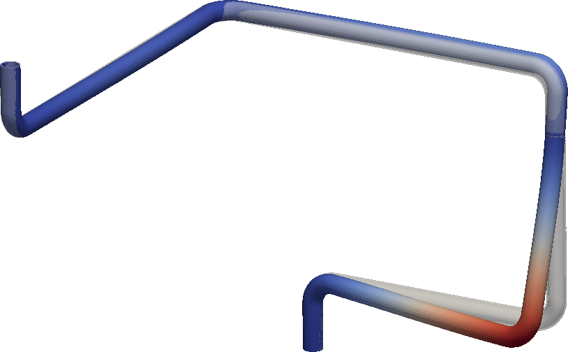
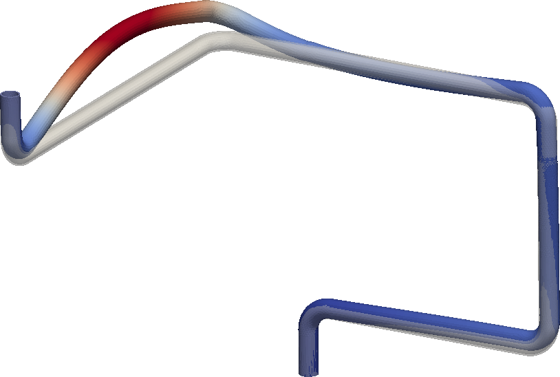
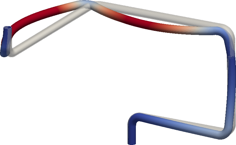
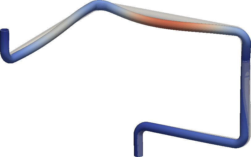
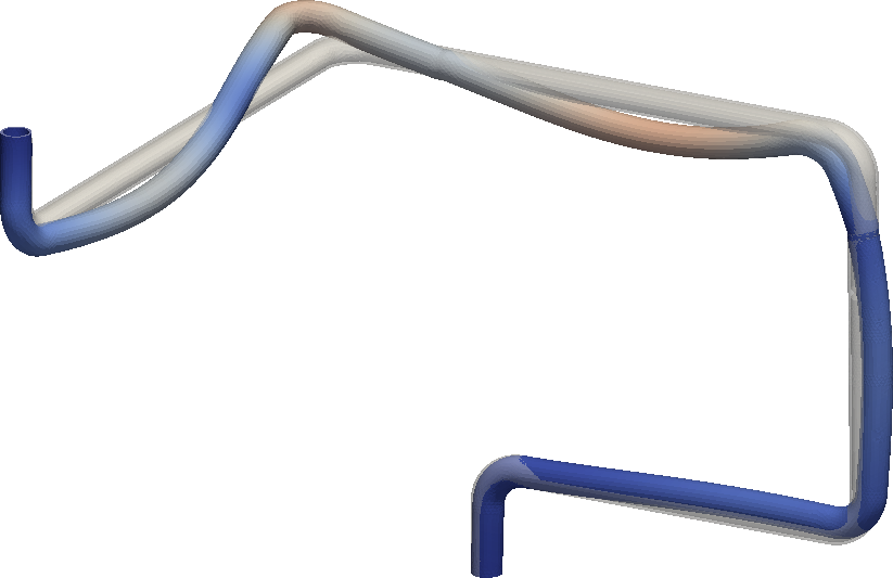
A real continuous solid has infinite modes of oscillation. A discretized one has three times the number of nodes modes of oscillation. In any case, one is usually interested only in a few of them, namely those with the lower frequencies because they take most of the energy with them. Each mode has two associated parameters called modal mass and excitation parameter that reflect how “important” the mode is regarding the absorption of energy from an external oscillatory source. Usually a couple of dozens of modes are enough to take up more than 90% of the earthquake energy. Figure\ [-@fig:modes] shows the first six natural modes of a sample piping section.

::::: {#fig:modes} {width=50%} {width=50%}

{width=50%} {width=50%}

{width=50%} {width=50%}

First six natural oscillation modes for a piping section. :::::

These first modes that take up most of the energy are then used to take into account the earthquake load. There are several ways of performing this computation, but the ASME\ III code states that the method known as SRSS (for Square Root of Sum of Squares) can be safely used. This method mixes the eigenvectors with the floor response spectra through the eigenvalues and gives an spatial (actually nodal) distribution of three accelerations (one for each direction) that, when multiplied by the density give a vector of a distributed force (in units of Newton per cubic millimeter for example) which is statically equivalent to the load coming from the postulated earthquake.

::::: {#fig:acceleration} {width=80%}

{width=80%}

{width=80%}

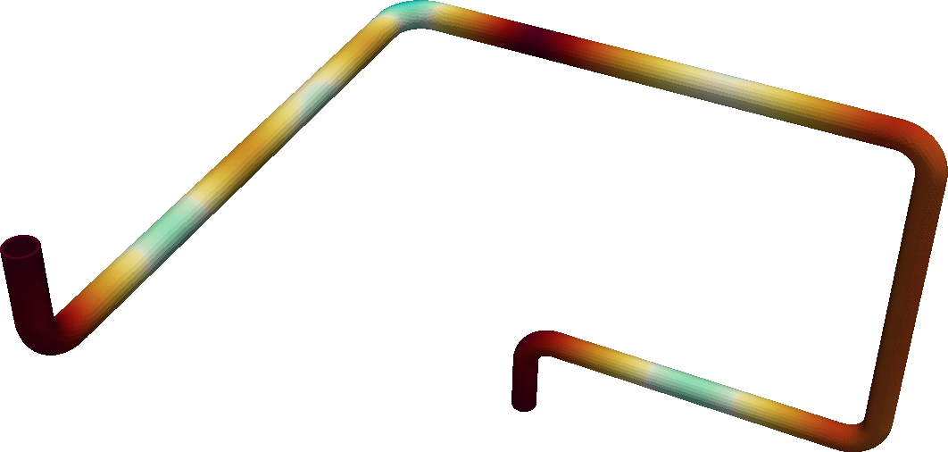
The equivalent accelerations for the piping section of [@fig:modes] for the spectra of\ [@fig:spectrum]. :::::

The ASME code says that these accelerations (depicted in [@fig:acceleration]) are to be applied twice. Once with the original sign and once with all the elements with the opposite sign during two seconds of the transient each time.

Linearity (not yet linearization)

Even though we did not yet discuss it in detail, we want to solve an elastic problem subject to an internal pressure condition, with a non-uniform temperature distribution that leads to both thermal stresses and variations in the mechanical properties of the materials. And as if this was not enough, we want to add at some instants a statically-equivalent distributed load that comes from a design earthquake. This last point means that at the transient instant where the stresses (from the fatigue’s point of view) are maximum we have to add the distributed loads that we computed from the seismic spectra to the other thermal and pressure loads. But we have a linear elastic problem (well, we still do not have it but we will in\ [@sec:break]), so we might be tempted exploit the problem’s linearity and compute all the effects separately and them sum them up to obtain the whole combination. We may thus compute just the stresses due to the seismic loads and then add them up to the stresses of any instant of the transient, in particular to the one with the highest ones. After all, in linear problems the result of the sum of two cases is the results of the sum of the cases, right? Wrong.

Let us jump out of our nuclear piping problem and step back into the general finite-element theory ground for a moment (remember we were going to jump back and forth). Assume you want to know how much your dog weights. One thing you can do is weight yourself (let us say you weight 81.2\ kg), then grab your dog and weight yourself and your dog (let us say you and your dog weight 87.3\ kg). Do you swear your dog weights 6.1\ kg plus/minus the scale’s uncertainty? I can tell you that the weight of two individual protons and two individual neutrons in not the same as the weight of an\ $alpha$ particle. Will not there be a master-pet interaction that renders the weighting problem non-linear?

Let us both (i.e. you and me) make an experiment. Grab a FEM program of your choice (mine is CAEplex) and load a 1mm $\times$ 1mm $\times$ 1mm cube. Set any values for the Young Modulus and Poisson ratio as you want. I chose\ $E=200$MPa and\ $\nu=0.28$. Restrict the three faces pointing to the negative axes to their planes, i.e.

• in face “left” ($x<0$), set null displacement in the $x$ direction ($u=0$),
• in face “front” ($y<0$), set null displacement in the $y$ direction ($v=0$),
• in face “bottom” ($z<0$), set null displacement in the $z$ direction ($w=0$).

Now we are going to create and compare three load cases:

a. Pure normal loads (https://caeplex.com/p?d8f) b. Pure shear loads (https://caeplex.com/p?b494) c. The combination of A & B (https://caeplex.com/p?989)

The loads in each cases are applied to the three remaining faces, namely “right”, “back” and “top,” and their magnitude in Newtons are:

\begin{center}
\rowcolors{2}{black!10}{black!0}
\begin{tabular}{l|ccc|ccc|ccc}
&
\multicolumn{3}{c|}{face “right” ($x>0$)} &
\multicolumn{3}{c|}{face “back” ($y>0$)} &
\multicolumn{3}{c}{face “top” ($z>0$)} \\

&
$F_x$ &
$F_y$ &
$F_z$ &
$F_x$ &
$F_y$ &
$F_z$ &
$F_x$ &
$F_y$ &
$F_z$ \\

\hline

Case A, pure normal & +10 &  0  &   0 &    0 & +20 &  0   &   0 &   0 & +30 \\
Case B, pure shear  &   0 & +15 & -15 &  +25 &   0 & -5   & -15 & +25 & +30 \\
Case C, combination & +10 & +15 & -15 &  +25 & +20 & -5   & -15 & +25 & +30 \\
\end{tabular}
\end{center}

<table>
 <tr>
  <th></th>
  <th colspan="3">face “right” ($x>0$)</th>
  <th colspan="3">face “right” ($x>0$)</th>
  <th colspan="3">face “right” ($x>0$)</th>
 </tr>  
 <tr>
  <th></th>
  <th>$F_x$</th>
  <th>$F_y$</th>
  <th>$F_z$</th>
  <th>$F_x$</th>
  <th>$F_y$</th>
  <th>$F_z$</th>
  <th>$F_x$</th>
  <th>$F_y$</th>
  <th>$F_z$</th>
 </tr>
 <tr>
  <td>Case A, pure normal</td>
  <td>+10</td><td>0</td><td>0</td><td>0</td><td>+20</td><td>0</td><td>0</td><td>0</td><td>+30</td>
 </tr>
 <tr>
  <td>Case B, pure shear</td>
  <td>0</td><td>+15</td><td>-15</td><td>+25</td><td>0</td><td>-5</td><td>-15</td><td>+25</td><td>0</td>
 </tr>
 <tr>
  <td>Case C, combination</td>
  <td>+10</td><td>+15</td><td>-15</td><td>+25</td><td>+20<td>-5</td><td>-15</td><td>+25</td><td>+30</td>
 </tr>
</table>

In the first case, the principal stresses are uniform and equal to the three normal loads. As the forces are in Newton and the area of each face of the cube is 1mm², the usual sorting leads to

divert(-1) $$ \begin{align} \sigma{1A} &= 30~\text{MPa} \ \sigma{2A} &= 20~\text{MPa} \ \sigma_{3A} &= 10~\text{MPa} \ \end{align} $$ divert(0)

$$ \sigma{1A} = 30~\text{MPa} $$ $$ \sigma{2A} = 20~\text{MPa} $$ $$ \sigma_{3A} = 10~\text{MPa} $$

::::: {#fig:cube} {#fig:cube-shear width=50%}

{#fig:cube-full width=50%}

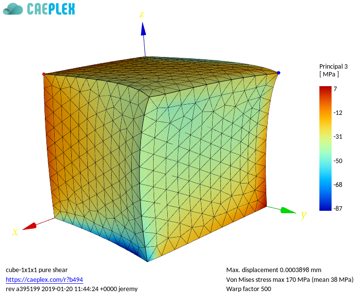
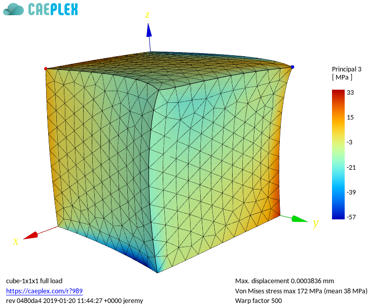
Spatial distribution of principal stress\ 3 for cases\ B and\ C. If linearity applied, case\ C would be equal to case\ B plus an constant. :::::

In the second case, the principal stresses are not uniform and have a non-trivial distribution. Indeed, the distribution of\ $\sigma_3$ obtained by CAeplex is shown in\ [@fig:cube-shear]. Now, if we indeed were facing a fully linear problem then the results of the sum of two inputs would be equal to the sum of the individual inputs. And\ [@fig:cube-full], which shows the principal stress\ 3 of case\ C is not the result from case\ B plus any of the three constants from case\ A. Had it been, the color distribution would have been exactly the same as the scale goes automatically from the most negative value in blue to the most positive value in red. And 7+30\ $\neq$ 33. Alas, it seems that there exists some kind of unexpected non-linearity (the feared master-pet interaction?) that prevents us from from fully splitting the problem into simpler chunks.

So what is the source of this unexpected non-linear effect in an otherwise nice and friendly linear formulation? Well, probably you already know it because after all it is almost high-school mathematics. But I learned it way after college when facing a real engineering problem and not just back-of-the-envelope pencil-and-paper trivial exercises.

Recall that principal stresses are the eigenvalues of the stress tensor. And the fact that in a linear elastic formulation means that the stress tensor of case\ C above is the sum of the individual stress tensors from cases\ A and B does not mean that their eigenvalues can be summed (think about it!). Again, imagine the eigenvalues and eigenvectors of cases A & B. Got it? Good. Now imagine the eigenvalues and eigenvectors for case\ C. Should they sum up? No, they should not! Let us make another experiment, this time with matrices using Octave or whatever matrix-friendly program you want.

First, let us create a 3$\times$3 random matrix $R$ and then multiply it by its transpose\ $R^T$ to obtain a symmetric matrix\ $A$ (recall that the stress tensor is symmetric):

octave> R = rand(3); A = R*R'
A =

   2.08711   1.40929   1.31108
   1.40929   1.32462   0.57570
   1.31108   0.57570   1.09657

Do the same to obtain another 3$\times$3 symmetric matrix\ B:

octave> R = rand(3); B = R*R'
B =

   1.02619   0.73457   0.56903
   0.73457   0.53386   0.37772
   0.56903   0.37772   0.53141

Now compute the sum of the eigenvalues first and then the eigenvalues of the sum:

octave> eig(A)+eig(B)
ans =

   0.0075113
   0.8248395
   5.7674016

octave> eig(A+B)
ans =

   0.049508
   0.782990
   5.767255

octave:36>

Did I convince you? More or less, right? The third eigenvalue seems to fit. Let us not throw all of our beloved linearity away and dig in further into the subject. There are still two important issues to discuss which can be easily addressed using fresh-year linear algebra (remember, do not fear math!). First of all, even though principal stresses are not linear with respect to the sum they are linear with respect to pure multiplication. Once more, think what happens to the the eigenvalues and eigenvectors of a single stress tensor as all its elements are scaled up or down by a real scalar. They are the same! So, for example, the Von Mises stress (which is a combination of the principal stresses) of a beam loaded with a force\ $\alpha \cdot \vec{F}$ is\ $\alpha$ times the stress of the beam loaded with a force\ $\vec{F}$. Please test this hypothesis by playing with your favorite FEM solver an play. Or even better, take a look at the stress invariants $I_1$, $I_2$ and $I_3$ (you can search online or peek into the source code of Fino and grep for the routine called fino_compute_principal_stress()) and see (using paper and pencil!) how they scale up if the individual elements of the stress tensor are scaled by a real factor\ $\alpha$.

The other issue is that even though in general the eigenvalues of the sum of two matrices are not the same as the eigenvalues of the matrix sum, there are some cases when they are. In effect, if two matrices\ $A$ and\ $B$ commute, i.e. their product is commutative

$$ A \cdot B = B \cdot A $$ then the sums of their eigenvalues are equal to the eigenvalues of the sums. In order for this to happen, both\ $A$ and\ $B$ need to be diagonalizable using the same basis. That is to say, the diagonalizing matrix\ $P$ such that $P^{-1} A P$ is diagonal is the same that renders\ $P^{-1} B P$ also diagonal. What does this mecanically mean? Well, if case\ A has loads that are somehow “independent” from the ones in case\ B, then the principal stresses of the combination might be equal to the sum of the individual principal stresses. A notable case is for example a beam that is loaded vertically in case\ A and horizontally in case\ B. I dare you to grab your FEM program one more time, run a test and picture the eigenvalues and eigenvectors of the three cases in your head.

The infinite pipe revisited after college

3D full

Quarter

2 grados

2D axysimmetric

1D collocation

struct vs unstruct

1st vs 2nd

complete vs incomplete (hexa)

ASME stress linearization (not linearity!)

Two (or more) materials

open source! que hacen los programas? NADIE SABE

Young and Poisson

two cubes

A parametric tee

Bake, shake and break

Fatigue

In air

In water

Conclusions

Back in College, we all learned how to solve engineering problems. But there is a real gap between the equations written in chalk on a blackboard (now probably in the form of beamer slide presentations) and actual real-life engineering problems. This chapter introduces a real case from the nuclear industry and starts by idealising the structure such that it has a known analytical solution that can be found in textbooks. Additional realism is added in stages allowing the engineer to develop an understanding of the more complex physics and a faith in the veracity of the FE results where theoretical solutions are not available. Even more, a brief insight into the world of evaluation of low-cycle fatigue using such results further illustrates the complexities of real-life engineering analysis.

• use your imagination
• practise math
• start with simple cases first
• grasp the dependence of results with independent variables
• keep in mind there are other methods beside finite elements
• within the finite element method, there is a wide variety of complexity in the problems that can be solved
• follow the “five whys rule” before compute anything, probably you do not need to
• use engineering judgment and make sure understand the “wronger than wrong” concept
• play with your favourite FEM solver (mine is https://caeplex.com) solving simple cases, trying to predict the results and picturing the stress tensor and its eigenvectors in your imagination

dnl errors and uncertainties: model parameters (is E what we think? is the material linear?), geometry (does the CAD represent the reality?) equations (any effect we did not have take account), discretization (how well does the mesh describe the geometry?)

---

1. A former boss once told me “I need the CFD” when I handed in some results. I replied that I did not do computational fluid-dynamics but computed the neutron flux kinetics within a nuclear reactor core. He joked “I know, what I need are the Colors For Directors, those pretty coloured figures along with your actual results.”
2. Please say “modeling” not “simulation.”