pipe-linearized/pipe-linearized.md

Introduction

The main objective of this report is to analyze the convergence of the ASME linearized stresses (membrane and membrane plus bending) in a pressurized infinitely-long circular pipe. This problem was chosen because

1. it is a typical problem tackled analytically in undergraduate courses in mechanical engineering (at least the displacements and stresses, not the ASME linearization),
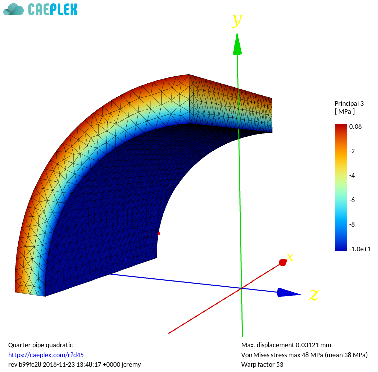
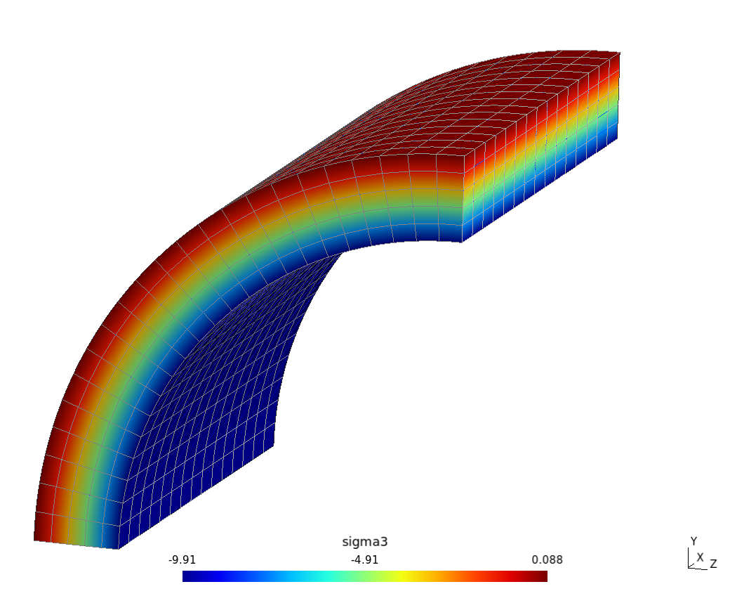
2. it can be easily solved using standard finite-element tools ([@fig:quarter-caeplex]) so it serves as a benchmark problem, and
3. there is a practical interest to compare stress analysis results from general piping systems to the canonical case of the infinite pipe.

{#fig:quarter-caeplex width=70%}

In this work, the term convergence is taken as the study of how the linearized stresses computed with a finite-element method change with respect to the number of elements through the pipe thickness. Briefly, this technical report

• analytically obtains the ASME-linearized (membrane and membrane plus bending) stresses for an infinite pipe subject to an uniform internal pressure,
• serves as a benchmarking test, comparing the results obtained by the free and open-source finite-element tool Fino and the analytical solution,
• shows how multi-freedom boundary conditions can be used to simplify the restriction of the rigid-body degrees of freedom in the case of null axial displacement and radial-only displacements,
• illustrates how parametric runs can be performed in Fino,
• analyzes the convergence of the ASME-linearized stresses with respect to the mesh coarseness,
• explores the differences between first and second-order elements regarding errors and computational efforts,
• compares the errors (with respect to the analytical solutions) obtained by using linear and quadratic elements as a function of the computational effort,
• quantitatively and qualitatively address the differences obtained in using both first and second-order elements.

For the finite-element computations, only tetrahedral unstructured grids are used to avoid biasing the results by having elements with edges parallel to the coordinate axis. Even more, the stress classification lines do no need to pass through any actual node of the grid. The software used to solve the finite-element formulation ([@sec:about]) allows the initial and end point of the stress classification lines to be arbitrary points of the domain. A parametric run is performed and the results are both qualitatively and quantitatively analyzed. A number of interesting conclusions are summarized in [@sec:conclusions]. The appendices that follow dive into further advanced and optional topics.

{#fig:struct width=60%}

It should be noted that the objective of this report is to study a very simple problem as thoroughly as possible in order to have a sound understanding of the underlying mechanical phenomena. There is absolutely no need to employ finite-element analysis to solve an infinite pressurized pipe. However, finite-elements ought to be employed to analyze any real piping network such as the one depicted in [@fig:cad1].

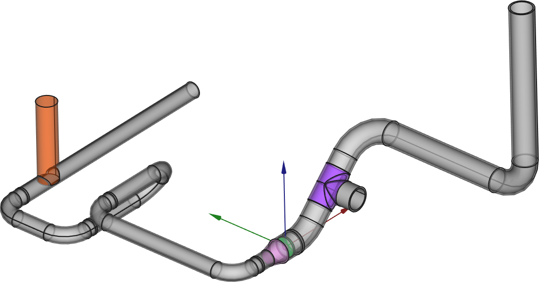{#fig:cad1}

About Fino

Fino is a free and open source tool that uses the finite-element method to solve

• steady-state thermo-mechanical problems, or
• steady or transient heat conduction problems, or
• modal analysis problems.

It is particularly designed to handle complex dependence of material properties (i.e. temperature-dependent properties). It can also perform parametric or optimization runs. The domain over which the problem is solved should be a grid generated by Gmsh. The material properties and boundary conditions may involve arbitrary dependence of space associated to physical entities defined in the mesh.

Fino follows, amongst others, the UNIX philosophy. Fino is a back-end aimed at advanced users. For an easy-to-use web-based front-end with Fino running in the cloud, see CAEplex.

Fino is a free (“Free” both as in “free speech” and in “free beer.”) and open source finite-element analysis tool Fino developed from scratch by Seamplex. From our point of view, only open source software¹ should be employed in solving engineering problems. A cognizant engineer cannot rely on privative software and be certain that the results are accurate, exact or even valid enough to draw an educated conclusion out of them. Any reasonable engineering system cannot depend on black boxes.

{width=25%}

Problem

Let us consider an infinite pipe (i.e. a cylinder) of internal radius $a$ and external radius $b$ with uniform mechanical properties---Young modulus $E$ and Poisson’s ratio $\nu$---subject to an internal uniform pressure $p$. We would like to compute the linearized membrane and membrane plus bending stresses according to ASME VIII Section 5 [@asme8div2, annex 5-A]. To obtain a numerical solution with the finite-element method, let us fix the numerical values of the parameters as follows

\begin{align*} dnl b &= \SI{esyscmd(echo “INCLUDE pipe-linearize/problem.was\nPRINT b” )}{\milli\meter} \ dnl a &= \SI{esyscmd(echo “INCLUDE pipe-linearize/problem.was\nPRINT a” )}{\milli\meter} \ dnl E &= \SI{esyscmd(echo “INCLUDE pipe-linearize/problem.was\nPRINT 1e-3*E” )}{\giga\pascal} \ dnl \nu &= esyscmd(echo “INCLUDE pipe-linearize/problem.was\nPRINT %.2f nu” ) \ dnl p &= \SI{esyscmd(echo “INCLUDE pipe-linearize/problem.was\nPRINT p” )}{\mega\pascal} \ b &= esyscmd(echo “INCLUDE pipe-linearize/problem.was\nPRINT b” )~\text{mm} \ a &= esyscmd(echo “INCLUDE pipe-linearize/problem.was\nPRINT a” )~\text{mm} \ E &= esyscmd([[echo “INCLUDE pipe-linearize/problem.was\nPRINT 1e-3E” | wasora - | xargs]])~\text{GPa} \ \nu &= esyscmd(echo “INCLUDE pipe-linearize/problem.was\nPRINT %.2f nu” ) \ \end{align} which correspond to a esyscmd(grep inch pipe-linearize/problem.was ) carbon steel pipe according to ASME B36-10M [@asmeb36]. Again, for the sake of numerical results, we fix the internal pressure to

$$ p = esyscmd(echo “INCLUDE pipe-linearize/problem.was\nPRINT p” )~\text{MPa} $$ that is a typical pressure found in nuclear power plants (so ASME III applies).

Reference analytical solution

Given the cylindrical symmetry of the problem, there is only one independent variable, namely the radial coordinate $r$. Moreover, there are only two displacement fields that need to be considered: the axial $u_a®$ and the radial $u_r®$. The former is identically zero due to the fact that the cylinder is infinite (plane strain condition). The equilibrium of momentum along the radial direction $r$ is

$$ \frac{d\sigma_r}{dr} + \frac{\sigmar® - \sigma\theta®}{r} = 0 $${#eq:equilibrium}

Defining the strains as

\begin{align} \epsilon_r &= \frac{dur}{dr} \ \epsilon\theta &= \frac{u}{r} \end{align} and the stresses as

\begin{align} \sigma_r &= \frac{E}{(1-\nu)(1-2\nu)} \cdot \Big[ (1-\nu) \cdot \epsilonr + \nu \cdot \epsilon\theta \Big] \ \sigma_\theta &= \frac{E}{(1-\nu)(1-2\nu)} \cdot \Big[ \nu \cdot \epsilon_r + (1-\nu) \cdot \epsilon_r \Big] \ \end{align} then the differential equation [-@eq:equilibrium] can be casted in terms of the axial displacement $u_r®$ as

$$ \frac{d^2 u}{dr^2} + \frac{1}{r} \cdot \frac{du}{dr} - \frac{u}{r^2} = 0 $$ that has the general solution

$$ u® = c_1 \cdot r + \frac{c_2}{r} $$

For the boundary conditions of the particular problem that the radial stress should be equal to the negative of the internal pressure² at $r=a$ and null at $r=b$, namely

$$ \begin{cases} \sigma_r(a) &= -p\ \sigma_r(b) &= 0 \end{cases} $$ the axial displacement has the particular solution

$$ u_r® = p \cdot \frac{1+\nu}{E} \cdot \frac{a^2}{b^2-a^2} \cdot \left[ 1-2\nu + \frac{b^2}{r^2} \right]\cdot r $$ and the stresses the radial, tangential (hoop) and axial (longitudinal) stresses are

$$ \sigmar® = \frac{p \cdot a^2}{b^2-a^2} \cdot \left( 1 - \frac{b^2}{r^2}\right) $$ {#eq:sigmar} $$ \sigma\theta® =\frac{p \cdot a^2}{b^2-a^2} \cdot \left( 1 + \frac{b^2}{r^2}\right) $$ {#eq:sigmatheta} $$ \sigma_l® = 2\nu \cdot \frac{p \cdot a^2}{b^2-a^2} $${#eq:sigmal}

Stress linearization

According to the ASME VIII code [@asme8div2], a stress classification line should be chosen to compute the linearized stresses. Theses SCLs should be normal to iso-stress lines, which in this case may be any line radial from $r=a$ to $r=b$. The ASME code defines that each element of the membrane stress tensor $\text{M}$ is

\begin{equation} \text{M}{ij} = \frac{1}{b-a} \cdot \int{a}^{b} \sigma_{ij}® \, dr \end{equation} \noindent for $i=x,y,z$ and $j=x,y,z$. Having computed the nine values (of which only six are different) of such tensor, different kind of scalar membrane stresses can be obtained depending on how a single scalar stress “intensity” is computed out of the nine tensor elements. In particular we take into account the Tresca,³ Von Mises and the three principal membrane stresses. As all the shear stresses are zero, $\sigma_l$, $\sigmar$ and $\sigma\theta$ happen to also be the principal stresses with

\begin{align} \sigma1 &= \sigma\theta \ \sigma_2 &= \sigma_l \ \sigma_3 &= \sigma_r \end{align}

So the membrane stresses to be considered are

\begin{align} \text{M}1 &= \frac{1}{b-a} \cdot \int{a}^{b} \sigma_\theta® \, dr \ \text{M}2 &= \frac{1}{b-a} \cdot \int{a}^{b} \sigma_l® \, dr \ \text{M}3 &= \frac{1}{b-a} \cdot \int{a}^{b} \sigmar® \, dr \ \text{M}\text{tresca} &= \max\Big{ \left| \text{M}_1 - \text{M}_2 \right|, \left| \text{M}_2 - \text{M}_3 \right|, \left| \text{M}_3 - \text{M}1 \right| \Big} \ \text{M}\text{vonmises} &= \sqrt{ \frac{(\text{M}_1-\text{M}_2)^2 + (\text{M}_2-\text{M}_3)^2 + (\text{M}_3-\text{M}_1)^2}{2}} \end{align}

In particular, replacing the stress distribution of the infinite pipe given by [@eq:sigmal; @eq:sigmar; @eq:sigmatheta] and carrying out the integrals, the principal membrane stresses are

\begin{align} \text{M}_1 &= {{a\,p}\over{b-a}} \ \text{M}_2 &= {{2\,a^2\,\nu\,p}\over{b^2-a^2}} \ \text{M}_3 &= {{a^2\,\left(2\,b-{{b^2+a^2}\over{a}}\right)\,p}\over{\left(b-a\right)\,\left(b^2-a^2\right)}} \end{align}

\medskip

The other linearized stress, namely the membrane plus bending stress tensor \text{MB}---again according to ASME VIII Annex 5-A---is

$$ \text{MB}{ij} = \text{M}{ij} \pm \frac{6}{(b-a)^2} \cdot \int{a}^{b} \sigma{ij}® \cdot \left( \frac{a+b}{2}-r\right) \, dr $${#eq:mb} where the sign should be taken such that the resulting combined scalar stress (i.e. Tresca, Von Mises, etc.) represents the worst-case scenario. As before, the membrane plus bending scalar stresses are

\begin{align} \text{MB}1 &= \text{M}{1} \pm \frac{6}{(b-a)^2} \cdot \int{a}^{b} \sigma\theta® \cdot \left( \frac{a+b}{2}-r\right) \, dr \ \text{MB}2 &= \text{M}{2} \pm \frac{6}{(b-a)^2} \cdot \int_{a}^{b} \sigma_l® \cdot \left( \frac{a+b}{2}-r\right) \, dr \ \text{MB}3 &= \text{M}{3} \pm \frac{6}{(b-a)^2} \cdot \int_{a}^{b} \sigmar® \cdot \left( \frac{a+b}{2}-r\right) \, dr \ \text{MB}\text{tresca} &= \max\Big{ \left| \text{MB}_1 - \text{MB}_2 \right|, \left| \text{MB}_2 - \text{MB}_3 \right|, \left| \text{MB}_3 - \text{MB}1 \right| \Big} \ \text{MB}\text{vonmises} &= \sqrt{ \frac{(\text{MB}_1-\text{MB}_2)^2 + (\text{MB}_2-\text{MB}_3)^2 + (\text{MB}_3-\text{MB}_1)^2}{2}} \end{align}

For the infinite pipe case, $\text{MB}_1$ is maximum and $\text{MB}_2$ is minimum if we take the positive sign in [@eq:mb]. The integral in the expression for $\text{MB}_2$ above vanishes. The principal membrane plus bending stresses are then

\begin{align} \text{MB}_1 &= \displaystyle{{6\,a^2\,\left({{b^3+\left(2\,a\,\log a+a\right)\,b^2-a^2\,b}\over{2\,a}}-{{2\,b^2\,\log b+b^2}\over{2}}\right)\,p}\over{\left(b-a\right)^2\,\left(b^2-a^2\right)}}+{{a\,p}\over{b-a}} \ \text{MB}_2 &= \displaystyle{{2\,a^2\,\nu\,p}\over{b^2-a^2}} \ \text{MB}_3 &= \displaystyle{{6\,a^2\,\left({{2\,b^2\,\log b+b^2+2\,a\,b}\over{2}}-{{b^3+\left(2\,a\,\log a+a\right)\,b^2+a^2\,b}\over{2\,a}}\right)\,p}\over{\left(b-a\right)^2\,\left(b^2-a^2\right)}}+{{a^2\,\left(2\,b-{{b^2+a^2}\over{a}}\right)\,p}\over{\left(b-a\right)\,\left(b^2-a^2\right)}} \end{align}

For the particular parameters fixed in [@sec:problem], the numerical values for the theoretical linearized membrane and membrane plus bending scalar stresses are

divert(-1) \begin{align} \text{M}_\text{tresca} &= \SI{esyscmd(grep -A1 ev(Mtresca pipe-linearize/analytical.txt | tail -n 1 | tr -d ‘ ’ | awk -F) ‘{printf(“%.4f”, $2) }’)}{\mega\pascal} \ \text{M}\text{vonmises} &= \SI{esyscmd(grep -A1 ev(M_vonmises pipe-linearize/analytical.txt | tail -n 1 | tr -d ‘ ’ | awk -F) ‘{printf(“%.4f”, $2) }’)}{\mega\pascal} \ \text{M}_1 &= \SI{esyscmd(grep -A1 ev(M_1 pipe-linearize/analytical.txt | tail -n 1 | tr -d ‘ ’ | awk -F) ‘{printf(“%.4f”, $2) }’)}{\mega\pascal} \ \text{M}_2 &= \SI{esyscmd(grep -A1 ev(M_2 pipe-linearize/analytical.txt | tail -n 1 | tr -d ‘ ’ | awk -F) ‘{printf(“%.4f”, $2) }’)}{\mega\pascal} \ \text{M}_3 &= \SI{esyscmd(grep -A1 ev(M_3 pipe-linearize/analytical.txt | tail -n 1 | tr -d ‘ ’ | awk -F) ‘{printf(“%.4f”, $2) }’)}{\mega\pascal} \ \end{align} and \begin{align} \text{MB}_\text{tresca} &= \SI{esyscmd(grep -A1 ev(MBtresca pipe-linearize/analytical.txt | tail -n 1 | tr -d ‘ ’ | awk -F) ‘{printf(“%.4f”, $2) }’)}{\mega\pascal} \ \text{MB}\text{vonmises} &= \SI{esyscmd(grep -A1 ev(MB_vonmises pipe-linearize/analytical.txt | tail -n 1 | tr -d ‘ ’ | awk -F) ‘{printf(“%.4f”, $2) }’)}{\mega\pascal} \ \text{MB}_1 &= \SI{esyscmd(grep -A1 ev(MB_1 pipe-linearize/analytical.txt | tail -n 1 | tr -d ‘ ’ | awk -F) ‘{printf(“%.4f”, $2) }’)}{\mega\pascal} \ \text{MB}_2 &= \SI{esyscmd(grep -A1 ev(MB_2 pipe-linearize/analytical.txt | tail -n 1 | tr -d ‘ ’ | awk -F) ‘{printf(“%.4f”, $2) }’)}{\mega\pascal} \ \text{MB}_3 &= \SI{esyscmd(grep -A1 ev(MB_3 pipe-linearize/analytical.txt | tail -n 1 | tr -d ‘ ’ | awk -F) ‘{printf(“%.4f”, $2) }’)}{\mega\pascal} \ \end{align} respectively. divert(0)

\begin{align} \text{M}_\text{tresca} &= esyscmd(grep -A1 ev(Mtresca pipe-linearize/analytical.txt | tail -n 1 | tr -d ‘ ’ | awk -F) ‘{printf(“%.4f”, $2) }’)~\text{MPa} \ \text{M}\text{vonmises} &= esyscmd(grep -A1 ev(M_vonmises pipe-linearize/analytical.txt | tail -n 1 | tr -d ‘ ’ | awk -F) ‘{printf(“%.4f”, $2) }’)~\text{MPa} \ \text{M}_1 &= esyscmd(grep -A1 ev(M_1 pipe-linearize/analytical.txt | tail -n 1 | tr -d ‘ ’ | awk -F) ‘{printf(“%.4f”, $2) }’)~\text{MPa} \ \text{M}_2 &= esyscmd(grep -A1 ev(M_2 pipe-linearize/analytical.txt | tail -n 1 | tr -d ‘ ’ | awk -F) ‘{printf(“%.4f”, $2) }’)~\text{MPa} \ \text{M}_3 &= esyscmd(grep -A1 ev(M_3 pipe-linearize/analytical.txt | tail -n 1 | tr -d ‘ ’ | awk -F) ‘{printf(“%.4f”, $2) }’)~\text{MPa} \ \end{align} and \begin{align} \text{MB}_\text{tresca} &= esyscmd(grep -A1 ev(MBtresca pipe-linearize/analytical.txt | tail -n 1 | tr -d ‘ ’ | awk -F) ‘{printf(“%.4f”, $2) }’)~\text{MPa} \ \text{MB}\text{vonmises} &= esyscmd(grep -A1 ev(MB_vonmises pipe-linearize/analytical.txt | tail -n 1 | tr -d ‘ ’ | awk -F) ‘{printf(“%.4f”, $2) }’)~\text{MPa} \ \text{MB}_1 &= esyscmd(grep -A1 ev(MB_1 pipe-linearize/analytical.txt | tail -n 1 | tr -d ‘ ’ | awk -F) ‘{printf(“%.4f”, $2) }’)~\text{MPa} \ \text{MB}_2 &= esyscmd(grep -A1 ev(MB_2 pipe-linearize/analytical.txt | tail -n 1 | tr -d ‘ ’ | awk -F) ‘{printf(“%.4f”, $2) }’)~\text{MPa} \ \text{MB}_3 &= esyscmd(grep -A1 ev(MB_3 pipe-linearize/analytical.txt | tail -n 1 | tr -d ‘ ’ | awk -F) ‘{printf(“%.4f”, $2) }’)~\text{MPa} \ \end{align} respectively. See [@sec:maxima] and [@sec:wasora] for the input files used to compute both the integrals and the numerical values, either using Maxima (symbolic integration) or wasora @wasoradesc.

Parametric finite-element analysis solution

In principle, the problem can be solved as a bi-dimensional plane-strain case. Even more, it is actually a one-dimensional problem with radial dependence only. Nevertheless, we solve a full three-dimensional pipe because we are interested in using the same set of methods and tools we would use in a real-case piping system. We do not even use any half or quarter symmetry but the full 360º annuli.

In order to study the convergence of the linearized stresses computed using the stresses obtained in a finite-element solution, the free and open source tool Fino---which gives the three-dimensional displacement field $[u(\mathbf{x}),v(\mathbf{x}),w(\mathbf{x})]$ and the corresponding stress tensor distribution---is used. The model geometry is first modeled and then meshed using the free and open source tool Gmsh [@gmsh]. The former consists of a cylinder with radii $a<b$ and a length $\ell=2(b-a)$ (as illustrated in [@fig:cylinder]) which was directly built using the constructive solid modeling primitives provided by Gmsh through the OpenCASCADE library ([@fig:cylinder]). The latter is generated parametrically over $n=1,\dots,6$, which indicates the number of expected elements through the pipe wall thickness $b-a$.

{#fig:cylinder width=35%}

Even though the cylinder is a rather simple and symmetric geometry, the grids are fully unstructured in order to avoid biased results that might correspond to a particular choice of the grid structure. It is also because of this reason that a full cylinder is modeled instead of just half or a quarter cylinder so there are no element edges parallel to the coordinate axes. In particular, both first and second-order tetrahedra are used for each value of $n$, giving rise thus to the analysis of twelve different FEM cases. The computational implementation uses the GNU M4 processor called from Fino to expand macros in a Gmsh geometry file template with the particular values of $a$, $b$, $n$ and the mesh order ([@sec:gmsh]).

The origin $(0,0,0)$ of the coordinate system is located at the cylinder’s barycenter, while the main axis corresponds to the cartesian $x$ axis, as illustrated in [@fig:cylinder]. The internal cylindrical face is subject to a uniform pressure $p$. Due to the fact that we are modeling an infinite cylinder, the external annuli which are parallel to the $y$-$z$ plane should have a null axial displacement ($u=0$) to recover the plane-strain conditions. Moreover, the displacements can only be radial so these faces are subject to the condition, remembering that the cylinder’s axis is located at $y=z=0$, that

$$v(x,y,z) \cdot z - w(x,y,z) \cdot y = 0$${#eq:radial}

See [@sec:radial] for a detailed derivation of this expression. These three boundary conditions are applied over two different faces, namely

• compression pressure $p$ in the internal cylindrical face, and
• null axial displacement $u=0$ and only radial displacement $v z - w y = 0$ in the two external axial plane surfaces.

\noindent can be easily implemented in Fino as shown in [@sec:fino]. Note that even though the two conditions in the second bullet correspond to Dirichlet (or essential) boundary conditions, only the first one $u=0$ is exactly enforced (up to the error of the iterative linear solver). The second one corresponds to a multi-freedom Dirichlet boundary condition and is implemented using a penalty method and it is thus only approximately imposed.⁴

Parametric grids

define(n_grids, esyscmd(grep PARAMETRIC pipe-linearize/pipe.fin ))

By expanding the macros of the Gmsh input template shown in [@sec:gmsh] for the parameter $n=1,\dots,6$ that represents the number of elements along the pipe wall thickness, the grids shown in [figures @fig:mesh1]--[-@fig:meshn_grids] are obtained. It should be noted that the number and distribution of elements is exactly the same in the first and second-order cases. However, not only is the number of nodes different but also the new second-order nodes (i.e. the nodes located along each of the the six edges the tetrahedra have) are placed on the curved surfaces of the cylinder. Thus, the original first-order tetrahedra are slightly “distorted” to better represent the continuous geometry in the second-order case. In any case, this distortion is so slight that each case cannot be graphically distinguished even for the coarser case. Nevertheless, this effect is present and is illustrated in the extremely coarse grids presented in [@fig:distorted]. The extra cost of this better geometrical representation is a greater number of nodes, which in turn leads to an increase in the computational effort needed to solve the associated finite-element problem as discussed in [@sec:resources]. Even though quadratic iso-parametric (i.e. standard) elements can better represent circles, they are still approximations. One need to switch to iso-geometric elements for that end.

divert(-1) forloop(i, 1, n_grids, [[ if(output_format, html, {width=80%}, \begin{figure}[p] \begin{center}\includegraphics[width=80%]{pipe-mesh-i.png}\end{center} \caption{\label{fig:meshi}Mesh for $n=i$} ]]) divert(0)

dnl ]])

dnl ]])

dnl ]])

dnl ]])

dnl ]])

dnl ]])

dnl ]])

dnl ]])

dnl ]])

dnl ]])

dnl ]])

dnl ]])

dnl ]])

:::: {#fig:mesh12} {#fig:mesh1 width=90%}

{#fig:mesh2 width=90%}

::::

::::

::::

::::

::::

::::

::::

::::

::::

::::

::::

::

:::: {#fig:mesh34} {#fig:mesh3 width=90%}

{#fig:mesh4 width=90%}

::::

::::

::::

::::

::::

::::

::::

::::

::::

::::

::::

::

:::: {#fig:mesh56} {#fig:mesh5 width=90%}

{#fig:mesh6 width=90%}

Parametric grids with\ $n$ elements through the pipe thickness. ::::

{#fig:distorted}

Displacements

The finite-element solver gives a vector field of displacements $[u(\mathbf{x}),v(\mathbf{x}),w(\mathbf{x})]$ in each of the three Cartesian directions $x$, $y$ and $z$, respectively. Due to the cylindrical symmetry, the only non-zero displacements will be $v(\mathbf{x})$ and $w(\mathbf{x})$ which, furthermore, will be related in such a way that only radial net displacements occur. Given the radial nature of the three-dimensional geometry, the radial displacement $u_r®$ should be compared with

$$ \sqrt{\left[v(x,r \cos \theta, r\sin\theta)\right]^2 + \left[w(x,r \cos \theta, r\sin\theta)\right]^2} $$ for any $-\ell/2 \leq x \leq +\ell/2$, $a \leq r \leq b$ and azimuthal angle $\theta$. It should be noted that the grid is fully unstructured, so there is no particular choice of $x$ and $\theta$ than can give different results, say because there are element edges aligned with the coordinate axis. To simplify the extraction of the numerical data, we can take either $v(0,r,0)$ or $w(0,0,r)$ as a representative measure of the radial displacement $u_r®$.

Fino allows the displacements $[u(\mathbf{x}),v(\mathbf{x}),w(\mathbf{x})]$ (and the stresses) to be evaluated at any arbitrary point $\mathbf{x}$, i.e. they are real continuous functions of space and not just scattered values [@milonga-design]. The figures in this and the following sections show these full continuous functions of the finite-element solutions as interpolated by the shape functions. [@Fig:ur] compares the analytical solution of the radial displacement $u_r®$ with the numerical solutions for different combinations of mesh order and $n$ as obtained by Fino. It can be seen that for the second-order grid, a low value of $n$ seems to be more accurate than the finer first-order case.

{#fig:ur}

Stresses

Let us now switch to analyze the stresses, where the difference between first and second-order grids is even more evident. Depending on how the finite-element code averages nodal values from the gradient of the displacements---which are discontinuous across element interfaces---there might be slight differences in the actual results. But in essence, we can see in [@fig:sigmar; @fig:sigmal; @fig:sigmatheta] that again, quadratic elements beat linear ones even with for coarser grids. This is especially true for $\sigma_r$ that when evaluated at $r=a$ should be $\sigma_r(a)=-p=-10~\text{MPa}$ according to [@eq:sigmar]. We need to recall that the finite-element formulation does not strictly fulfill natural (i.e. Neuman or load) boundary conditions. It only can approximate them, with the approximation being better with refined meshes.

{#fig:sigmar}

:::: {#fig:sigmas-l-theta} {#fig:sigmal}

{#fig:sigmatheta}

Longitudinal and tangential normal stresses ::::

The reason of this behavior is that in first-order tetrahedra, the derivatives of the shape functions are uniform in space. Therefore, the stresses (that depend on the gradient of the displacements) are uniform throughout each element. The values of these uniform stresses are somehow an average of the contribution of each of the four nodes of the tetrahedron. For those elements that are in the bulk of the domain, the processes of computing the stresses at the nodes---which depends on the finite-element code implementation but in general involves averaging back the contributions of each of the elements that share a node---gives reasonable results because some of the element would contribute by defect and some by excess to the final nodal average. But those nodes that are located in the internal (external) faces of the pipe will have elements contributing only with values by excess (defect). Therefore, first-order elements will mostly give incorrect stresses at $r=a$ and $r=b$, overestimating them in the former and underestimating them in the latter. This is exactly the behavior of the first-order stresses obtained in [@fig:sigmar;@fig:sigmal;@fig:sigmatheta]. Second-order elements still have non-uniform spatial derivatives and they can recover (almost⁵) the real values for the stresses at the nodes located in the boundary of the domain.

Linearized stresses

We can now analyze how the results of the linearization of the stresses according to ASME VIII [@asme8div2, annex 5-A]. Note that Fino allows the location of the SCLs to be arbitrary, in the sense that the end points do not need to be actual nodes of the grids. See [@sec:fino] for details of the input files used to compute the linearized stresses, where the definition of the SCLs are given as continuous coordinates and not as references to any particular grid node.

Figures [-@fig:M_tresca]--[-@fig:MB_3] show the membrane $\text{M}$ and membrane plus bending $\text{MB}$ stresses for different compositions of the stress tensor (Tresca, Von Mises and the three principal stresses) for $n=1,\dots,n_grids$ compared to the analytical solutions obtained in [@sec:analytical]. The vertical axes span a $\pm5\%$ range around the value given by analytical solution. It can be seen that $\text{M}$ converges faster than $\text{MB}$.

This last statement can be explained using the uniform-derivative reasoning explained in [@sec:stresses]. As the membrane stress is essentially an average along the stress classification line, the excess and defect errors committed by the first-order grids in $r=a$ and $r=b$ almost cancel out. Therefore, the error for computing $\text{M}$ with linear elements is not that relevant. However, the membrane plus bending stress is a first-order momentum of the stress distribution. This time, the deviations do not cancel out and they both contribute with the same sign to the value of linearized stress. It is this effect that gives such a slow convergence for $\text{MB}$.

:::: {#fig:tresca} {#fig:M_tresca}

{#fig:MB_tresca}

::::

::::

::::

::::

:::

:::: {#fig:vonmises} {#fig:M_vonmises}

{#fig:MB_vonmises}

Linearized Von Mises stresses ::::

:::: {#fig:principal1} {#fig:M_1}

{#fig:MB_1}

Linearized principal stresses\ 1 ::::

:::: {#fig:principal2} {#fig:M_2}

{#fig:MB_2}

::::

::::

::::

::::

::::

::::

:

:::: {#fig:principal3} {#fig:M_3}

{#fig:MB_3}

Linearized principal stresses\ 3 ::::

Computational resources

As evident as it it that second-order elements give far superior results than linear ones, any fair analysis needs to compare solutions that involve similar amounts of computational efforts both in random-access memory and number of floating-point operations---otherwise we would end up comparing apples and oranges. That is to say, we might be comparing results from a run that takes one week with a one-second execution and then conclude that the first scheme gives better results than the second. Yes, it does, but it is not a fair comparison.

Roughly speaking, the CPU and memory consumption depend non-linearly on the size of the discretized problem, which is three times the number of nodes and not (at least directly) on the number of elements of the mesh. Remember that the latter are the same for a fixed value of $n$ both in first and second-order grids (see again the exaggerated [@fig:distorted]). Furthermore, the stiffness matrix of a second-order finite-element formulation is less sparse than the one corresponding to a similar first-order problem (though if now the number of nodes was kept constant to have similar matrix sizes, the former would have less elements so the effort needed to build it would be surprisingly lower for the second-order matrix) rendering the solution of the linear system of equations even more difficult.

In effect, the number of elements as a function of $n$ is the same for both grids, as it can seen in [@fig:elements-vs-n]. But the number of nodes is far higher in the second-order grid for the same $n$ ([@fig:nodes-vs-n]). This leads to more CPU and memory, as shown in [@fig:cpu-vs-n; @fig:memory-vs-n].

:::: {#fig:ele-nodes-vs-n} {#fig:elements-vs-n}

{#fig:nodes-vs-n}

::::

::::

::::

::::

::::

::

:::: {#fig:cpu-mem-vs-n} {#fig:cpu-vs-n}

{#fig:memory-vs-n}

CPU time and memory vs.\ $n$ ::::

Error as a function of CPU time

So, on the one hand, for a fixed $n$, second-order elements give far better results than linear elements. On the other hand, the former consume far more computational resources than the latter. Therefore, in order to compare apples and apples, in principle the comparison of results should be performed by fixing the number of nodes (and, again, not the number of elements) as discussed above. But given that the problem we are solving does have analytical solutions, we can also analyze the errors associated to each of the finite-element formulations as a function of the computational effort.

Figures [-@fig:error-M-vs-cpu] and [-@fig:error-MB-vs-cpu] show a log-log plot of the absolute value of the difference between the linearized stresses computed using Fino and the analytical solution of [@sec:analytical] as a function of the CPU time needed to solve the finite-element formulation. It can be seen that the membrane stress $\text{M}$ can be reasonably solved using first-order elements, as the first-order error is comparable to the second-order error for similar amounts of CPU time. However, for the evaluation of the bending stresses $\text{MB}$, linear elements give very poor results when compared to quadratic elements for the same computational effort.

These two figures quantitatively illustrate the effect discussed in [@sec:linearized] that the membrane and the membrane plus bending stress are zero and first-order moments respectively. In the former case, the excess and defect errors of the extreme nodes cancel out whereas in the latter case they do not.

:::: {#fig:errors-vs-n} {#fig:error-M-vs-cpu}

{#fig:error-MB-vs-cpu}

Errors vs.\ $n$ ::::

Conclusions

There are a few conclusion we can draw out of the results obtained in this report:

• Engineering problems ought not to be solved using black-boxes (i.e. privative software whose source code is not freely available).
• The pressurized infinite pipe has only one independent variable (the radius $r$) and one primary dependent variable (the radial displacement $u_r$).
• The problem has analytical solution for the radial displacement and the radial, tangential and axial stresses.
• There are no shear stresses, so these three stresses are also the principal stresses.
• Analytical expressions for the membrane and membrane plus bending stresses along any radial SCL can be obtained.
• The spatial domain can be discretized using linear or higher-order elements. In particular first and second-order elements have been used in this report.
• For the same number of elements, second-order grids need more nodes than linear ones, although they can better represent curved geometries.
• The discretized problem size depends on the number of nodes and not on the number of elements.
• The finite-element results for the displacements are similar to the analytical solution, with second-order grids giving better results for the same number of elements (this is expected as they involved far more nodes).
• The three stress distributions computed with the finite-element give far more reasonable results for the second-order case than for the first-order grid. This is qualitatively explained by the fact that first-order tetrahedra have uniform derivatives and such the elements located in both the external and external faces represent the stresses not at the actual faces but at the barycenter of the elements.
• Membrane stresses converge well for both the first and second-order cases because they represent a zeroth-order moment of the stress distribution and such the excess and defect errors committed by the internal and external elements approximately cancel out.
• Membrane plus bending stresses converge very poorly in first-order grids because the excess and defect errors do not cancel out because it is a first-order moment of the stress distribution.
• The computational effort to solve a given problem, namely the CPU time and the needed RAM depend non-linearly on various factors, but the most important one is the problem size which is three times the number of nodes in the grid.
• The error with respect to the analytical solutions as a function of the CPU time needed to compute the membrane stress is similar for both first and second-order grids. But for the computation of the membrane plus bending stress, first-order grids give very poor results compared to second-order grids for the same CPU time.

All in all, these are the two main conclusions:

1. Using second-order elements for the computation of ASME linearized stresses is (almost) mandatory.
2. Using just two elements along the pipe thickness is enough to attain convergence of the linearized stresses.

\appendix

\newpage

---

Multi-freedom boundary condition for radial-only displacements

To set the condition that in the external surfaces all displacement ought to be radially-symmetrical around the barycenter of the surface, a multi-freedom Dirichlet boundary condition needs to be set. That is to say, it is not the value of the actual displacements that is fixed but a certain relationship between the three displacements $u$, $v$ and $w$ and the spatial coordinates $x$, $y$ and $z$.

In effect, let $\mathbf{x_0}=[\pm\ell/2,0,0]$ be the location of the barycenter of the face where the condition is to be applied. To force all displacements to be only radial, we require the vectors $\mathbf{u}=[u,v,w]$ and $(\mathbf{x}-\mathbf{x_0})$ to have the same direction. Using the scalar product notation:

\begin{align} \mathbf{u} \cdot \left(\mathbf{x}-\mathbf{x}_0\right) &= | \mathbf{u} | \cdot | \left(\mathbf{x}-\mathbf{x}_0\right)| \ u \cdot (x-x_0) + v \cdot (y-y_0) + w \cdot (z-z_0) &= \sqrt{u^2 + v^2 + w^2} \cdot \sqrt{(x-x_0)^2 + (y-y_0)^2 + (z-z_0)^2} \end{align} and taking into account that

• $u=0$ because of the null axial displacement condition,
• $\mathbf{x_0}=[\pm\ell/2,0,0]$, and
• $x=\pm \ell/2$,

\noindent then by squaring both members of the equation, we can simplify this expression to

$$ (v y + w z)^2 = (v^2 + w^2) \cdot (y^2 + z^2) $$

Further algebraic manipulation leads to

\begin{align} (vy)^2 + 2 \cdot v y \cdot w z + (wz)^2 &= (vy)^2 + (vz)^2 + (wy)^2 + (wz)^2 \ 2 \cdot v y \cdot w z &= (vz)^2 + (wy)^2 \ 0 & = (vz - wy)^2 \end{align} from which [@eq:radial] follows.

\newpage

---

Host, codes, scripts and input files

The complete set of scripts and input files needed to run the cases discussed in this report can be found at

:::: {text-center} https://bitbucket.org/seamplex/pipe-linearize ::::

\medskip

The results shown in this report correspond to revision

esyscmd(cd pipe-linearize; git log -1)

\noindent and were obtained using the free-as-in-free-speech⁶ tools Gmsh and Fino using the following versions:

include(pipe-linearize/versions.txt)

These codes were executed on a host with the following features:

include(pipe-linearize/cpu.txt)

The complete case can be run by executing the following script:

include(pipe-linearize/run.sh)

Analytical solutions with Maxima

The reference solutions presented in [@sec:analytical] where computed from the theoretical stresses by symbolic integration using Maxima.

include(pipe-linearize/problem.max)

include(pipe-linearize/analytical.max)

The results are illustrated in the following terminal mimic:

$ maxima -b analytical.max
include(pipe-linearize/analytical.txt)dnl
$

Theoretical solutions with wasora

Instead of symbolic integration, adaptive numerical quadrature can be performed easily using wasora [@wasoradesc]. First, we put all the problem parameters in a file problem.was:

include(pipe-linearize/problem.was)

And then include this file from the main one analytical.was:

include(pipe-linearize/analytical.was)

$ wasora analytical.was
include(pipe-linearize/analytical.ppl)dnl
$

Geometry and mesh generation with Gmsh

include(pipe-linearize/pipe.geo.m4)

Parametric finite-element analysis with Fino

include(pipe-linearize/pipe.fin)

\newpage

---

References

---

1. And if it is free software, even better.
2. Exercise for the reader: why the negative of the pressure and not the pressure itself?
3. Even though recent revisions of the ASME VIII code dropped the Tresca criterion in favor of Von Mises, the former is still the main way of computing the stress “intensity” in ASME III.
4. The null axial displacement condition $u=0$ is a traditional Dirichlet boundary condition because the outward normal $\mathbf{\hat{n}}$ coincides with one of the three coordinate axes. In the general case, it should also be set as a multi-freedom Dirichlet boundary condition.
5. The rate of convergence of the stresses in the nodes located in the boundary of the domain is linear, while it is quadratic in the bulk.
6. And not just free as in “free beer”